
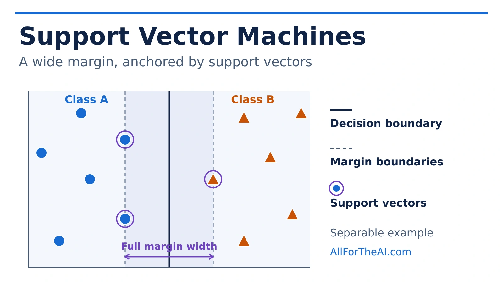
Support Vector Machines, usually shortened to SVMs, are supervised machine-learning methods used mainly for classification, although related methods can also perform regression and novelty detection.
An SVM tries to find a decision boundary that separates classes while leaving a useful margin between that boundary and the closest training examples.
Those influential training examples are called support vectors. This guide explains decision boundaries, margins, soft-margin classification, C, kernels, gamma, feature scaling, evaluation, and how SVM compares with other classical algorithms.
If supervised learning is new to you, start with Supervised Learning Explained before continuing.
Reviewed and updated October 3, 2026: This guide was reviewed for technical accuracy, learning-path structure, and current SVM terminology.
What Is a Support Vector Machine?
A Support Vector Machine is a supervised machine-learning method that learns a boundary between different classes of labeled training examples.
Imagine a dataset containing circles for Class A and squares for Class B. If the two groups can be separated, many different lines might divide them correctly. An SVM asks which boundary gives the classes an appropriate separation while balancing training errors and model complexity.
For a basic linear SVM, that means finding a separating hyperplane with a large margin around it. In two dimensions the boundary can be a line, in three dimensions it can be a plane, and in higher-dimensional feature spaces the general term is hyperplane.
A Simple SVM Example
Suppose we want to classify fruit using two features: weight and sweetness. Our labeled training data contains apples and oranges. Several lines might separate the groups correctly, but one may pass extremely close to examples on both sides while another leaves more room.
An SVM prefers a boundary according to its maximum-margin objective, while accounting for allowed classification errors when the data is not perfectly separable. It does not guarantee a universally “best” boundary; the fitted result depends on the objective, regularization settings, features, and training data.
Decision Boundaries, Margins, and Support Vectors
What Is the Decision Boundary?
A decision boundary separates regions of the feature space that the model assigns to different classes. For a binary problem, examples on one side may be classified as Class A and examples on the other as Class B.
What Is the Margin?
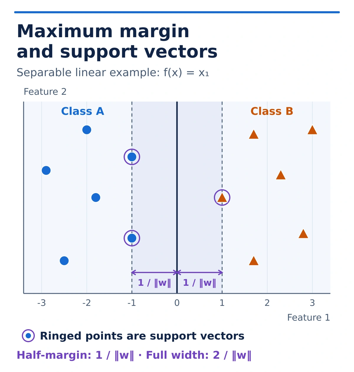
The margin is the space between the decision boundary and important nearby training examples. A larger margin can make a classifier less dependent on tiny changes around the separator, but the widest possible margin is not automatically the best model. Real data can contain overlap, noise, and unusual observations.
What Are Support Vectors?
Support vectors are training examples that play a direct role in defining the fitted SVM decision boundary. In the simple geometric picture, they are usually the examples closest to the margin or examples that violate it.
The full training dataset participates in the optimization that produces the fitted model. Support vectors are the subset that appears directly in the resulting decision function for a standard kernel SVM.
Hard-Margin vs Soft-Margin SVM
The simplest SVM picture assumes that the classes can be separated perfectly. This is the hard-margin idea. Real datasets rarely behave that cleanly: classes may overlap, labels may be wrong, measurements may be noisy, and some observations may be genuinely ambiguous.
A soft-margin SVM allows some observations to enter or cross the margin, or even be misclassified. The model balances maintaining a useful margin against avoiding too many or overly costly violations.
What Does C Mean in SVM?
C is an important regularization parameter. It controls how strongly the model penalizes training errors and margin violations. The scikit-learn SVM guide uses the same regularization framing.
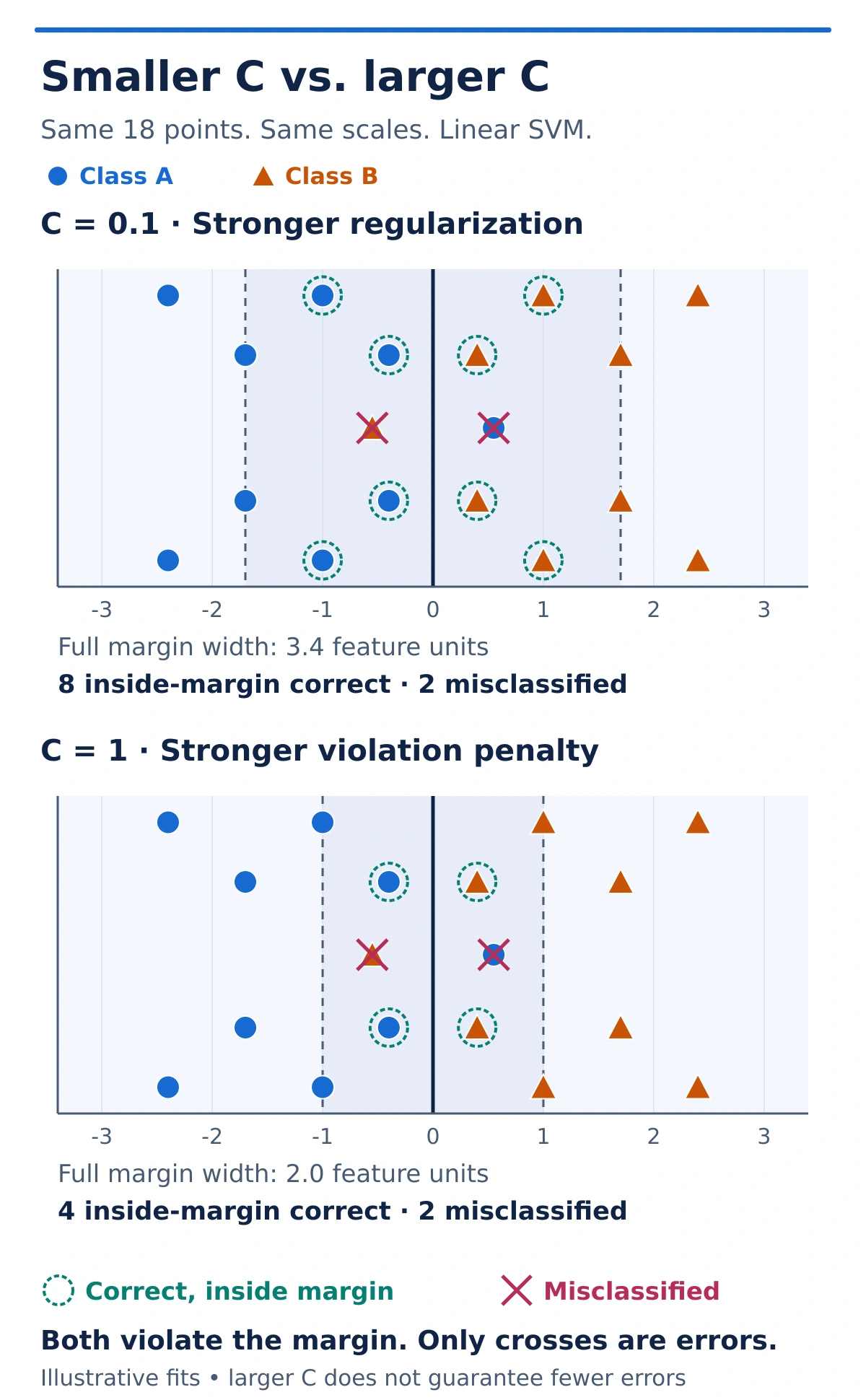
Smaller C applies stronger regularization: margin violations receive less weight relative to keeping the boundary simple, often allowing a wider margin. Larger C penalizes violations more strongly and can produce a tighter fit. A correctly classified point can still violate the margin; only points on the wrong side of the decision boundary are misclassified. Neither extreme is automatically better. Choose C with validation data or cross-validation rather than repeatedly checking the final test set.
Linear SVM and Nonlinear Classification
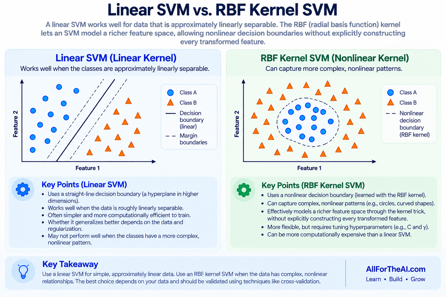
A linear SVM learns a linear boundary in the supplied feature space. Linear SVMs can work well when the classes are reasonably separable, when there are many features, and when the representation suits the problem. High-dimensional text classification is a classic example.
Not every problem has a useful straight-line boundary. One class might form a group in the center while another surrounds it. SVMs address such patterns with richer features or with kernels.
What Is the Kernel Trick?
A kernel lets an SVM model relationships corresponding to a richer feature space without explicitly calculating every coordinate of that space. Conceptually: original features → richer representation → linear separation in that representation → a nonlinear boundary when viewed in the original space.
The popular explanation that SVM simply “moves data into 3D” can help as a picture, but it is not the general computational story. Kernel methods can correspond to feature spaces with many dimensions without explicitly constructing them all.
Common SVM Kernels
- linear;
- polynomial;
- radial basis function, or RBF;
- sigmoid.
For beginners, the most important distinction is between linear and RBF kernels. A linear kernel fits a linear separator in the supplied representation. The RBF kernel permits more flexible, localized nonlinear boundaries.
What Does Gamma Mean?
For kernels such as RBF, gamma affects how localized the influence of individual training examples is. Lower gamma gives a broader influence; higher gamma makes that influence more local.
Very high gamma can follow the training data too closely; very low gamma can be too smooth. Consider gamma and C together during validation.
Why Feature Scaling Matters for SVM
Feature scaling is particularly important in many SVM workflows because the model’s geometry depends on distances or dot products. If one feature ranges from 18–80 and another from 20,000–200,000, their numerical scales can strongly affect the result even when the larger-number feature is not more meaningful.
Common approaches include standardization and min-max scaling. Prevent data leakage by splitting first, fitting the scaler on training data, and applying that learned transformation to validation and test data. See Data Preprocessing Explained and Training vs Testing Data.
How an SVM Classification Workflow Works
- Define the problem. Decide what class the model should predict.
- Prepare labeled examples. Supervised classification needs inputs paired with known targets.
- Split the data. Separate training, model-selection, and final test data.
- Preprocess the features. Fit learned transformations using development data only.
- Choose a setup. Begin with a linear SVM or a kernel such as RBF.
- Train the model. Learn the decision function from training examples.
- Tune carefully. Select
C, kernel, and applicablegammavalues through validation or cross-validation. - Evaluate once. Use untouched test data after development decisions are complete.
How Does SVM Handle More Than Two Classes?
SVM is easiest to explain with two classes, but practical implementations combine binary classifiers for multiclass problems. A common strategy is one-vs-one; some linear implementations use one-vs-rest. SVM is therefore not limited to two-class datasets.
Are SVM Outputs Probabilities?
Not automatically. A standard SVM naturally produces a decision score related to its learned decision function. Probability estimates require an additional calibration procedure and should not be treated as identical to the original score.
Other SVM Variants
Support Vector Regression
Support Vector Regression (SVR) adapts related support-vector ideas to numerical prediction, balancing tolerated prediction errors and model complexity.
One-Class SVM
One-Class SVM is a specialized method for novelty or outlier detection. It models a region containing typical examples and identifies observations that differ from it.
SVM Compared With Other Algorithms
SVM vs Logistic Regression
On narrow screens, scroll the table sideways. Keyboard users: focus the table region and use the left and right arrow keys.
| Concept | Logistic Regression | Linear SVM |
|---|---|---|
| Main goal | Model a classification probability relationship | Learn a margin-based classifier |
| Natural output | Probability-oriented | Decision score |
| Linear boundary | Yes | Yes |
| Nonlinear option | Changed features or model formulation | Kernel SVM is a common extension |
| Scaling | Often useful | Particularly important in many workflows |
Neither model is universally better. The right choice depends on the representation, dataset size, probability and interpretability requirements, and validation performance. Read Logistic Regression Explained.
SVM vs K-Nearest Neighbors
KNN predicts from nearby stored examples and can make prediction more expensive as the dataset grows. SVM learns a decision function; for a standard kernel SVM, that fitted function depends on support vectors. Both methods can be sensitive to feature scaling. Read K-Nearest Neighbors Explained.
SVM vs Decision Trees and Random Forest
Trees classify through feature-based splits and generally require less concern about arbitrary numeric scaling. A small decision tree can be easier to interpret, while Random Forest combines many trees for a more robust ensemble. SVM uses margin-based geometry, can use kernels, and often requires more careful scaling and tuning. Continue with Decision Trees Explained or Random Forest Explained.
When SVM Can Work Well
- classification with a suitable linear or nonlinear boundary;
- high-dimensional feature spaces such as some text representations;
- moderately sized datasets with appropriate preprocessing;
- problems where a strong classical baseline is valuable.
These are potential strengths, not guarantees that SVM will outperform every alternative.
Limitations of Support Vector Machines
- Kernel SVMs can scale poorly: nonlinear training may become expensive as the number of samples grows, although linear implementations can scale much better. See the scikit-learn SVM user guide for implementation details.
- Scaling matters: poorly scaled features can distort the geometry.
- Tuning matters: kernel,
C, andgammachoices can materially change results. - Interpretability is limited: nonlinear boundaries are harder to explain as simple rules.
- Probabilities are not native: calibrated estimates require extra work.
- Noise and overlap complicate classification: soft margins help but do not remove the need for careful evaluation.
Class Imbalance and Evaluation
If one class is much rarer than another, accuracy alone can be misleading. Training may need class or sample weights, and evaluation should use metrics suited to the actual consequences of errors.
Use validation or cross-validation for model selection, then evaluate once on untouched test data. Learn more in Model Evaluation Metrics, Accuracy vs Precision vs Recall, Confusion Matrix Explained, and Overfitting vs Underfitting.
Frequently Asked Questions
What is an SVM in simple terms?
An SVM is a supervised method that learns a boundary between labeled classes while balancing a large margin against classification errors.
What are support vectors?
They are training examples that play a direct role in defining the fitted decision boundary.
Can SVM handle nonlinear data?
Yes. Kernel methods such as RBF allow nonlinear decision boundaries, although they add computational cost and tuning choices.
Is SVM always better than logistic regression?
No. They optimize different objectives and have different output, scaling, interpretability, and computational properties. Compare them with validation appropriate to the task.
Can SVM be used for regression?
Yes. Support Vector Regression is a related method for predicting numerical values.
What to Learn Next
You have now seen several supervised-learning algorithms. Next, switch paradigms and see how an unsupervised algorithm finds groups when no target labels are supplied.
For comparison, you can also revisit Logistic Regression, K-Nearest Neighbors, Decision Trees, or return to the Machine Learning Algorithms overview.