
Logistic Regression is a supervised classification method that estimates the probability of a class. It starts with a linear score, passes that score through the sigmoid function, and—when a hard decision is needed—compares the probability with a chosen threshold.
This guide uses spam detection as a running example. You will learn why the method has “regression” in its name, how it is trained, how to interpret its coefficients, how thresholds affect precision and recall, and when a different model may be a better choice. It follows Linear Regression Explained in the Machine Learning Algorithms Overview.
What Is Logistic Regression?
Logistic Regression is a supervised learning algorithm used primarily for classification. In binary classification, the target has two possible classes—for example, spam or not spam. The model estimates a probability for the designated positive class and can convert that probability into a class label.
In standard machine-learning terminology, Logistic Regression is a linear model for classification, despite its name. Its output is not an unrestricted number: the logistic, or sigmoid, function keeps the estimated probability between 0 and 1. See the scikit-learn Logistic Regression guide.
Why Is It Called Regression If It Classifies?
The name comes from what the model fits. Logistic Regression models a transformed probability—the log-odds, also called the logit—as a linear combination of the features. That regression-like linear relationship happens on the log-odds scale; the resulting probability can then support a classification decision.
This creates a useful bridge from Linear Regression: both models learn coefficients and an intercept, but Logistic Regression adds a link function that maps the linear result into a probability. Google’s learning sequence likewise introduces Logistic Regression after Linear Regression; see Google’s sigmoid explanation.
Algorithm vs Trained Logistic Model
Logistic Regression algorithm refers to the method used to define and fit the relationship. A trained Logistic Regression model is the fitted result: its learned coefficients and intercept can turn new feature values into estimated class probabilities.
From a Linear Score to a Probability
The central idea is a four-step pipeline. Each step stays readable on a small screen:
- Features: describe the email, such as whether it contains an urgent phrase or an unfamiliar link.
- Linear score: the model combines those feature values with its learned coefficients: z = b₀ + b₁x₁ + b₂x₂ + …
- Sigmoid: the function p = 1 / (1 + e−z) converts the unrestricted score into a probability between 0 and 1.
- Output: the result is the model-estimated probability that the email belongs to the positive class—in this example, spam.
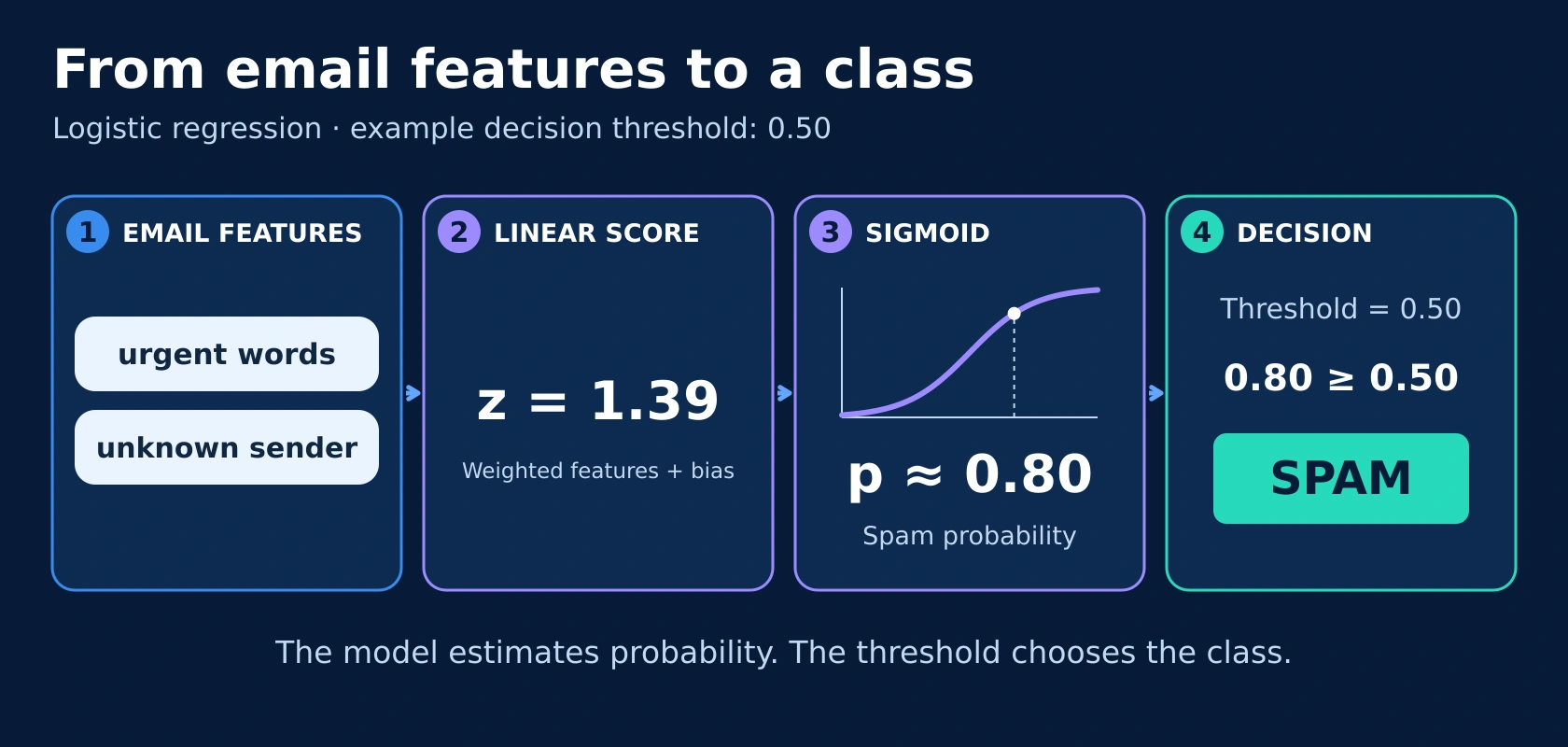
The score z can be any real number. The sigmoid compresses it into a value greater than 0 and less than 1. A score of 0 maps to 0.5; increasingly positive scores approach 1, while increasingly negative scores approach 0.
| Linear score z | Sigmoid probability p |
|---|---|
| −6 | 0.002 |
| −3 | 0.047 |
| 0 | 0.500 |
| 3 | 0.953 |
| 6 | 0.998 |
Worked Example: Classifying One Email
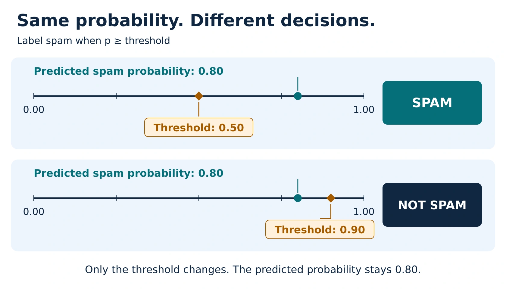
Suppose a trained spam model produces a linear score of z = 1.39 for one email. Passing that score through the sigmoid gives a predicted spam probability of about 0.80.
- With a threshold of 0.50, 0.80 is above the threshold, so the email is labeled spam.
- With a stricter threshold of 0.90, 0.80 is below the threshold, so the email is labeled not spam.
The features and coefficients behind 1.39 are omitted here so the example isolates the central idea: the model first estimates a probability, and the threshold is a separate decision rule. Google describes the same sequence as a linear equation followed by the sigmoid function. A predicted value such as 0.80 is a model estimate under the fitted model; it is not automatically proof of 80% real-world reliability.
Odds, Log-Odds, and the Logit
Odds and log-odds matter because they provide the scale on which Logistic Regression combines feature effects linearly. If the predicted probability is p, the odds are:
odds = p / (1 − p)
A probability of 0.75 corresponds to odds of 0.75 / 0.25 = 3, or 3-to-1. The logit is the natural logarithm of those odds:
logit(p) = log(p / (1 − p))
Logistic Regression assumes that this log-odds value can be represented adequately by a linear combination of the included features and transformations. Penn State’s STAT 504 lesson on binary Logistic Regression explains this logit link and the model’s assumptions in detail.
How Logistic Regression Works
- Define the target. Decide which class is encoded as 1—the positive class—and which is encoded as 0.
- Plan the data split. Establish training, validation, and untouched test data before learning transformations. See Training vs Testing Data.
- Prepare features safely. Fit preprocessing steps using training data, then apply them consistently. See Data Preprocessing and Feature Engineering.
- Fit coefficients. Training adjusts the intercept and feature coefficients to reduce a probability-based loss.
- Produce probabilities. New feature values create a linear score, which the sigmoid maps to a predicted probability.
- Evaluate and select. Compare model settings and thresholds on validation data using metrics that match the task.
- Test once. Evaluate the finalized approach on untouched test data before deployment or reporting.
How Logistic Regression Is Trained
Logistic Regression is typically fitted by maximum likelihood, which is equivalent to minimizing log loss for the usual binary formulation. Log loss evaluates the predicted probabilities, not just the final class labels. It gives a particularly large penalty to a confident prediction that is wrong.
Three ideas must remain separate:
- Training objective: log loss guides coefficient fitting.
- Decision threshold: converts probabilities into class labels when required.
- Evaluation metrics: measure probability quality, classification errors, or ranking performance.
Google’s Logistic Regression loss and regularization lesson explains why log loss is used instead of squared loss.
Regularization
Regularization discourages excessively large coefficients. It can improve stability and generalization, especially when features are numerous or correlated. L2 regularization shrinks coefficients, L1 can shrink some to zero, and Elastic Net combines L1 and L2. Scikit-learn’s Logistic Regression implementation supports these options and applies regularization by default, depending on the chosen settings and solver.
How to Interpret Logistic Regression Coefficients
A positive coefficient raises the modeled log-odds of the positive class as that feature increases, holding the other included features fixed. A negative coefficient lowers them. Exponentiating a coefficient gives an odds ratio: eβ represents the multiplicative change in the modeled odds for a one-unit increase in that feature, with the other included predictors held fixed.
Interpretation depends on units, feature encoding, interactions, transformations, regularization, and model specification. Strongly correlated predictors can make individual coefficients unstable even when overall prediction remains useful. Most importantly, a coefficient describes an association in the fitted model; it does not prove that the feature causes the outcome. Penn State provides worked coefficient and odds-ratio interpretations in its binary Logistic Regression notes.
Decision Thresholds
A probability is not yet a hard class decision. If a spam model returns 0.62, a threshold of 0.50 labels the message as spam, while a threshold of 0.70 labels it as not spam.
| Threshold change | Typical effect | Main trade-off |
|---|---|---|
| Lower threshold | More cases predicted positive | Recall often rises; false positives may rise |
| Higher threshold | Fewer cases predicted positive | Precision may rise; false negatives may rise |
0.5 is common, not universally optimal. Choose a threshold with validation data according to the relative costs of false positives and false negatives and the intended use of the model. Do not choose it by looking repeatedly at the final test set.
How to Evaluate Logistic Regression
No single metric is best for every classification problem. Use a combination that reflects the model output and the decision consequences:
| Measure | What it tells you |
|---|---|
| Log loss | How well the predicted probabilities align with the true labels; confident errors are penalized heavily. |
| Confusion matrix | The counts of true positives, false positives, true negatives, and false negatives at a chosen threshold. |
| Accuracy | The share of predictions that are correct; potentially misleading when classes are imbalanced or errors have unequal costs. |
| Precision | Among predicted positives, the share that are truly positive. |
| Recall | Among actual positives, the share detected by the model. |
| F1 score | The harmonic mean of precision and recall. |
| ROC-AUC | A threshold-independent summary of how well scores rank positives above negatives; useful in some settings, but not a complete evaluation. |
Continue with Model Evaluation Metrics, Accuracy vs Precision vs Recall, and Confusion Matrix Explained. Penn State also covers ROC curves and Logistic Regression diagnostics in STAT 504 Lesson 7.
Class Imbalance and Threshold Trade-offs
If one class is much rarer than the other, raw accuracy can look high even when the model barely identifies the minority class. Inspect the confusion matrix, precision, recall, and probability behavior for the classes that matter. Possible responses include appropriate resampling, class or sample weighting, collecting more representative data, and selecting a threshold aligned with the objective—but each must be validated without contaminating the test set.
When Is Logistic Regression Appropriate?
- The target is categorical, with binary classification as the clearest starting case.
- Observations are sufficiently independent for the way the model and evaluation are defined.
- The log-odds relationship can be represented adequately by the included features, transformations, and interactions.
- The features contain useful information for separating the classes.
- There is enough representative data for stable estimation and evaluation.
- A transparent linear baseline or probability estimate is useful.
Logistic Regression does not require the raw binary outcome to have a linear relationship with each feature. The linearity assumption applies to the log-odds. It also does not directly inherit ordinary Linear Regression’s normal-error or equal-variance assumptions. Scaling is not a universal mathematical requirement, but it can affect optimization, numerical stability, regularization, and comparisons between coefficients.
Common Problems and Limitations
- Misspecified log-odds relationship: nonlinear patterns may require transformations, interactions, or another model family.
- Multicollinearity: redundant predictors can destabilize individual coefficient interpretations.
- Separation and sparse data: near-perfect class separation or too few informative cases can drive unstable estimates; regularization may help.
- Outliers and influential observations: unusual feature combinations can affect the fitted coefficients.
- Class imbalance: default thresholds and accuracy may hide poor minority-class performance.
- Calibration: a value such as 0.80 is a predicted probability, not automatically a reliable “confidence score.” Calibration should be checked on suitable held-out data.
- Association is not causation: coefficient signs and odds ratios do not establish causal effects.
Scikit-learn’s probability calibration guide explains that reliable probability interpretation depends on calibration and model specification. Also watch for Overfitting vs Underfitting.
Binary and Multiclass Logistic Regression
Binary Logistic Regression
Binary Logistic Regression predicts between two categories and is the primary form taught in this guide. It provides the cleanest introduction to sigmoid probabilities, odds, log-odds, thresholds, and confusion-matrix errors.
Multinomial Logistic Regression
Multinomial Logistic Regression extends the idea to more than two unordered classes, producing probabilities across the possible categories. Scikit-learn documents both binary and multinomial formulations in its linear-model guide.
Ordinal Logistic Models
When categories have a natural order—such as low, medium, and high—ordinal Logistic Regression models are a related but distinct extension with additional assumptions. Do not assume that every standard binary or multinomial implementation is automatically an ordinal model.
Strengths and Trade-offs
| Strengths | Trade-offs |
|---|---|
| Useful, relatively efficient baseline for many classification tasks | A linear decision boundary may miss complex structure |
| Produces class-probability estimates | Probabilities still require calibration checks |
| Coefficients can support interpretation with care | Interpretation becomes difficult with correlated, transformed, or interacting features |
| Regularization can improve stability | Results depend on preprocessing, penalty, data quality, and model specification |
Claims that Logistic Regression is always fast, simple, or interpretable should be qualified. Training cost depends on dataset size, sparsity, solver, convergence, and multiclass setup. Interpretability depends on whether the features and specification make the coefficients meaningful.
Logistic Regression vs Linear Regression
| Question | Linear Regression | Logistic Regression |
|---|---|---|
| Primary task | Predict a continuous number | Estimate class probabilities for classification |
| Model output | Unrestricted numeric value | Probability between 0 and 1 |
| Core relationship | Outcome modeled linearly | Log-odds modeled linearly |
| Common training loss | Squared error | Log loss |
| Hard decision threshold | Usually not applicable | Optional and task-dependent |
| Typical evaluation | MAE, MSE/RMSE, R² | Log loss, confusion matrix, precision, recall, F1, and sometimes ROC-AUC |
Both models learn coefficients and an intercept. Logistic Regression’s sigmoid and logit link are what adapt the linear score to a probability-based classification task.
FAQ
Is Logistic Regression classification or regression?
In standard machine-learning usage, it is a classification method that estimates class probabilities. “Regression” refers to modeling log-odds as a linear function of the features.
Why does Logistic Regression use a sigmoid function?
The sigmoid maps any real-valued linear score into a value between 0 and 1, which can be interpreted as a model-estimated probability.
Is 0.5 always the best classification threshold?
No. The appropriate threshold depends on the cost of false positives and false negatives, the class distribution, and the real objective. Choose it using validation data.
Does a predicted probability equal confidence?
Not automatically. It is a probability produced by the fitted model. Treating it as a reliable confidence level requires evidence that the model is appropriately calibrated for relevant data.
Does Logistic Regression require normally distributed errors?
No. The normal-error and constant-variance assumptions of ordinary Linear Regression do not transfer directly. Logistic Regression instead models a binomial outcome through the logit link and assumes the log-odds structure is adequately specified.
Can Logistic Regression handle more than two classes?
Yes. Multinomial Logistic Regression extends the approach to more than two unordered classes. Binary Logistic Regression remains the best starting point for understanding the method.
Are Logistic Regression coefficients causal?
No. They describe conditional associations in the fitted model. Causal conclusions require an appropriate study design and causal assumptions beyond fitting Logistic Regression.
Continue Learning
Remember the sequence: features create a linear score, the sigmoid converts that score into a probability, and a task-specific threshold can turn the probability into a class label. Training, probability estimation, threshold choice, and final evaluation are related but separate steps.
The next lesson introduces rule-like splits that can capture nonlinear relationships without requiring a linear log-odds structure.