
Reviewed and updated October 3, 2026.
A decision tree is a supervised machine-learning model that learns a hierarchy of decision rules from training data, then follows those rules from a root node to a leaf to make a prediction.
Decision trees can predict categories, such as spam or not spam, and numerical values, such as a house price. Their step-by-step structure makes small trees easy to inspect, but unrestricted trees can overfit and become unstable. This guide explains both the intuition and the important limitations.
What is a decision tree?
A decision tree is part of supervised learning: it learns from examples that contain input features and a known target. During training, the algorithm searches for conditions that divide those examples into increasingly useful groups. The learned conditions form a tree.
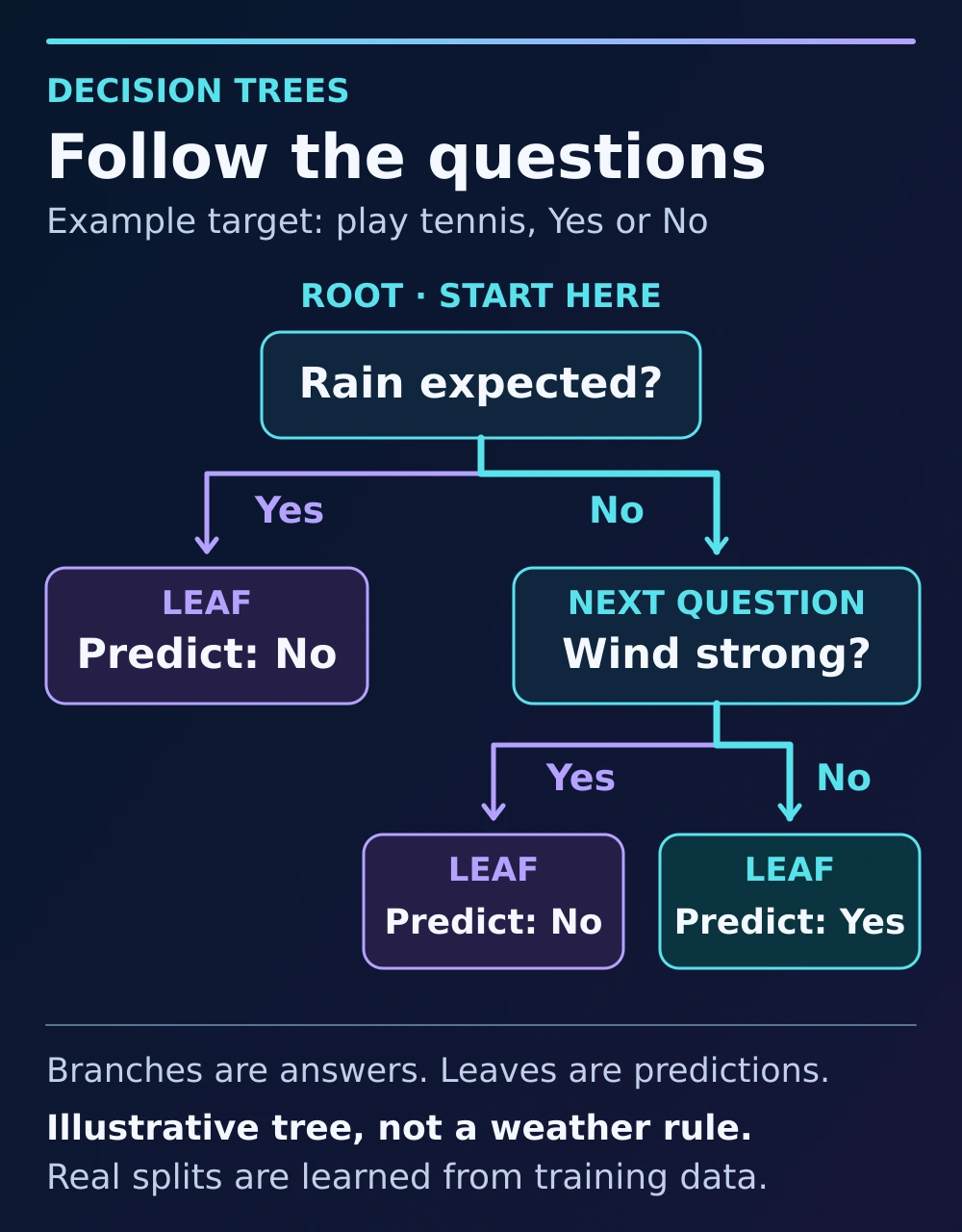
After training, a new example starts at the top of the tree. It follows one branch at each condition until it reaches a leaf containing the prediction. The developer chooses the training setup and complexity controls; the algorithm learns the particular splits from the data.
A learned machine-learning tree differs from a manually authored rule tree or flowchart: the learning algorithm selects splits from examples, while a person writes the conditions in a manual rule system. Both can look like branching diagrams, but their rules come from different processes.
Decision tree anatomy
- Root node: the first condition, where every prediction path begins.
- Internal or decision node: a later learned condition.
- Branch: the path produced by the result of a condition.
- Leaf or terminal node: the final prediction region.
- Depth: the greatest number of steps from the root to a leaf.
Imagine a small customer-churn tree. The root might ask whether account age is less than 12 months. One branch could then test recent support contacts. A leaf might predict “likely to churn.” Real trees usually evaluate numeric thresholds or encoded feature values rather than natural-language questions.
Classification trees and regression trees
On narrow screens, scroll the table sideways. Keyboard: focus the table region and use the left and right arrow keys.
| Tree type | What it predicts | Example |
|---|---|---|
| Classification tree | A category or class | Spam or not spam |
| Regression tree | A numerical value | House price |
A classification leaf can also provide estimated class probabilities based on the proportions of training examples that reached that leaf. A regression leaf outputs a representative numerical value determined by the training objective. The same tree-shaped idea therefore supports two different kinds of prediction.
How a decision tree is trained
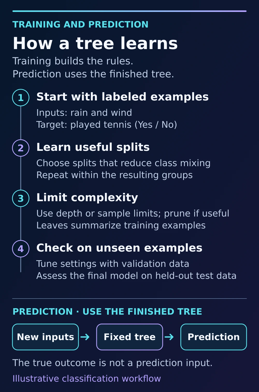
- Place the training examples at the root.
- Consider candidate features and split points.
- Measure how useful each candidate split would be.
- Choose a strong split according to the selected criterion.
- Divide the examples into child nodes.
- Repeat the process within each child node.
- Stop when a defined condition is reached.
Most practical tree-building methods are greedy: at each node they choose a locally strong split rather than testing every possible complete tree. This makes training manageable, but it does not guarantee the globally best tree.
How the “best split” is chosen
For classification, a useful split tends to create child nodes that are less mixed than the parent. If a parent contains an even mix of two classes, a split that produces one mostly-class-A child and one mostly-class-B child is useful.
On narrow screens, scroll the table sideways. Keyboard: focus the table region and use the left and right arrow keys.
| Criterion | Beginner interpretation |
|---|---|
| Gini impurity | How mixed the classes are in a node |
| Entropy | Another measure of class uncertainty or mixing |
| Information gain | How much a proposed split reduces that uncertainty |
Gini impurity is not an accuracy score, and neither Gini nor entropy is universally best. For regression, useful splits create groups whose target values are more similar within each resulting node. Common regression criteria measure reductions in errors such as squared error or absolute error.
How prediction works
Training builds the tree. Prediction uses the finished tree:
new example → root condition → branch → next condition → leaf → prediction
The tree does not ordinarily learn new splits each time it predicts. It applies the structure learned during training. This separation between training and inference matters when evaluating a model on validation, test, or real-world data.
Overfitting: the central limitation
An unrestricted tree can keep creating highly specific branches until it fits the training examples extremely closely. Training performance may rise while performance on unseen data gets worse. That is overfitting.
Tree complexity can be controlled with maximum depth, minimum samples required to split a node, minimum samples in a leaf, minimum improvement required for a split, and maximum leaves. Restricting complexity can improve generalization when a deeper tree is fitting noise, but too much restriction can cause underfitting. This is a practical example of the bias–variance tradeoff.
Pruning
Growing a tree creates candidate branches. Pruning removes branches whose extra complexity is not justified by improved generalization. Some methods limit growth in advance; others grow a larger tree and prune it afterward. The purpose is to balance fit against complexity.
Choose pruning strength and other complexity settings using a validation set or cross-validation, rather than training accuracy alone. Compare performance across candidate settings, then use a held-out test set for a final estimate after model selection. A simpler tree is useful when it generalizes better, not merely because it has fewer branches.
Interpretability—and where it breaks down
An individual shallow tree can often be visualized, followed node by node, and expressed as if/then-style rules. That makes its prediction path easier to inspect than many more complex models.
Decision trees are not automatically explainable in every practical setting. A very large tree can be difficult to reason about, and a visible prediction path does not prove that the model is fair, causal, or safe. High-stakes uses still require appropriate data governance, evaluation, human oversight, and domain expertise.
Why a single tree can be unstable
A single decision tree can have high variance: a small change in the training data may change an early split, producing a substantially different tree below it. That instability is one reason a single tree may perform inconsistently on new samples.
Random Forests address part of this weakness by training many varied trees and aggregating their predictions. The ensemble is less easy to inspect as one compact rule set, but it is often more stable than a single tree.
Preprocessing, missing values, and categories
Axis-aligned decision trees generally do not require feature standardization merely because variables use different numerical scales. This differs from distance-based methods such as K-nearest neighbors, where scale can strongly affect distance.
That does not mean decision trees require no data preprocessing. Data-quality problems, leakage, invalid values, unsupported feature types, and library-specific requirements still matter. Support for missing and categorical values depends on the implementation, so avoid blanket rules that trees always handle them automatically or always require one-hot encoding.
Advantages and limitations
Advantages
- Supports classification and regression
- Represents nonlinear relationships and interactions
- Usually needs little feature scaling
- Makes fast root-to-leaf predictions
- Small trees can be visualized and interpreted
Limitations
- Can overfit easily
- Can be unstable and high-variance
- Greedy training may miss the globally best tree
- Large trees lose interpretability
- Regression trees extrapolate poorly
- Axis-aligned splits may need many partitions
When is a decision tree useful?
A decision tree is worth testing when you have a supervised classification or regression problem—especially with tabular data—and value an inspectable baseline, nonlinear relationships, or limited scaling requirements. Illustrative tasks include customer-churn classification, equipment-failure classification, and house-price regression.
These are task examples, not claims that a particular company or high-stakes system uses a standalone tree. Model choice should be based on validated performance, error costs, data quality, fairness and safety requirements, and comparison with appropriate baselines using suitable evaluation metrics.
A note on feature importance
A fitted tree can report which features contributed strongly to its splitting structure, but importance is not causality. Impurity-based importance can also be misleading, so treat it as one diagnostic rather than proof that a feature causes the outcome.
Decision trees compared with nearby algorithms
For the broader map of model families, see Machine Learning Algorithms: A Beginner’s Guide.
On narrow screens, scroll the table sideways. Keyboard: focus the table region and use the left and right arrow keys.
| Algorithm | Core idea | Key distinction |
|---|---|---|
| Logistic regression | Estimates class probability using a linear relationship | Linear boundary |
| KNN | Uses nearby training examples | Distance-based |
| Decision tree | Partitions data with learned conditions | Rule/tree structure |
| Random Forest | Aggregates many varied trees | Ensemble |
| Support vector machine | Learns a separating boundary and margin | Boundary-based |
Frequently asked questions
Are decision trees only for classification?
No. Classification trees predict classes, while regression trees predict numerical targets.
Do decision trees always make yes/no splits?
No. Binary splits are common, but the exact branching behavior depends on the algorithm and implementation.
Do decision trees need feature scaling?
Usually not for ordinary axis-aligned threshold splits. Other preprocessing requirements still depend on the data and implementation.
Are decision trees always interpretable?
No. Shallow trees can be highly interpretable, but interpretability declines as a tree grows large and complex.
Authoritative references
- scikit-learn: Decision Trees — classification, regression, complexity control, pruning, and limitations.
- Google Machine Learning: Decision Trees — tree structure, splitting, training, and inference.
- Penn State STAT 508: Tree-Based Methods — construction, impurity, pruning, and ensemble context.
Next: from one tree to a forest
One tree is intuitive but can overfit and change sharply when the data changes. The logical next lesson is Random Forest Explained, which shows how combining many varied trees can reduce variance.
Need a refresher first? Review Overfitting vs Underfitting.