
Linear Regression is a supervised-learning method for predicting a numerical target from a linear combination of one or more input features. It is an excellent first algorithm to learn because every prediction can be traced to an equation, while its limitations introduce residuals, evaluation, diagnostics, and extrapolation.
Last reviewed and updated: September 13, 2026
This is the first algorithm-specific lesson after the Machine Learning Algorithms Overview. If features and targets are new to you, review Supervised Learning Explained and Dataset Fundamentals first.
What Is Linear Regression?
Linear Regression predicts a numerical target using a linear combination of feature values. With one feature, the fitted relationship can be drawn as a straight line. With several features, the same idea extends into more dimensions. Scikit-learn describes linear models with the general form ŷ = w₀ + w₁x₁ + … + wₚxₚ, where the fitted weights are coefficients and w₀ is the intercept. See scikit-learn’s linear-model guide.
A feature might be a home’s floor area, and the numerical target might be its price. The fitted model estimates an association between them. A regression relationship alone does not establish causation. Other variables, data-collection choices, or chance can explain an observed association.
Linear Regression Model vs Fitting Method
Linear Regression defines the form of the model: a numerical target is modeled as a linear combination of one or more features. Ordinary least squares (OLS) is a common fitting method that uses the training data to choose the coefficient and intercept values. The trained, or fitted, model is the resulting equation with those learned values. Different training datasets can therefore produce different fitted equations with the same Linear Regression model form.
The Linear Regression Equation
ŷ = b0 + b1x
- ŷ (“y-hat”) is the predicted target.
- x is the feature value.
- b₀ is the intercept.
- b₁ is the coefficient, or slope.
Worked Example: From Input to Residual
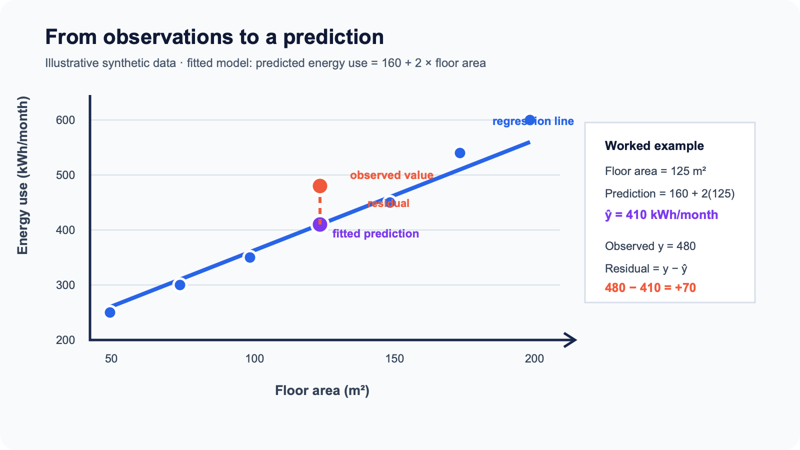
Suppose an illustrative fitted model predicts monthly energy use with ŷ = 160 + 2x, where x is floor area in square metres. For a 125 m² home, the prediction is ŷ = 160 + 2(125) = 410 kWh/month. If the observed energy use is 480 kWh/month, the residual is y − ŷ = 480 − 410 = +70 kWh/month. The positive residual means the observed value is 70 kWh/month above the fitted prediction.
For multiple features, the equation becomes ŷ = b₀ + b₁x₁ + b₂x₂ + … + bₚxₚ. Each feature contributes its value multiplied by its fitted coefficient.
Coefficients and Intercept
Coefficient
Holding the other included features constant, a coefficient describes how the model’s predicted target changes for a one-unit change in that feature.
Intercept
The intercept is the model’s predicted target when every included feature equals zero. Zero may fall outside the observed data or lack a useful real-world meaning.
Coefficients are often easier to inspect than the internal representations of more complex models, but interpretability is not automatic. Correlated, transformed, poorly measured, or hard-to-explain features can make coefficients difficult to interpret.
How Linear Regression Fits the Best Model
The standard version introduced here is ordinary least squares (OLS). The model predicts each training target, calculates the residual for each example, squares those residuals, and adds them. OLS chooses the coefficients that minimize this residual sum of squares. This is the objective used by scikit-learn’s LinearRegression. Read the scikit-learn LinearRegression reference.
Squaring prevents positive and negative residuals from canceling and gives larger errors more weight. OLS is the usual starting point, but other linear estimators use penalties, weights, or different loss functions.
What Is a Residual?
A residual is the observed target minus the model’s fitted prediction: eᵢ = yᵢ − ŷᵢ. A positive residual means the observed value is above the fitted prediction; a negative residual means it is below. Penn State’s STAT 501 notes use these vertical gaps to explain fitting and diagnose whether a linear model is adequate. See Penn State’s residual and assumptions lesson.
Step-by-Step Linear Regression Workflow
- Define the numerical target and features. Decide what number the model should predict and which inputs are available at prediction time.
- Split the data safely. Establish training, validation, and test roles before learning preprocessing choices. Review Training vs Testing Data.
- Prepare useful features. Fit learned transformations on training data only. See Data Preprocessing and Feature Engineering.
- Fit the equation. OLS estimates the intercept and coefficients by minimizing squared residuals.
- Evaluate on unseen data. Use validation data or cross-validation during development, then reserve the test set for the finalized approach.
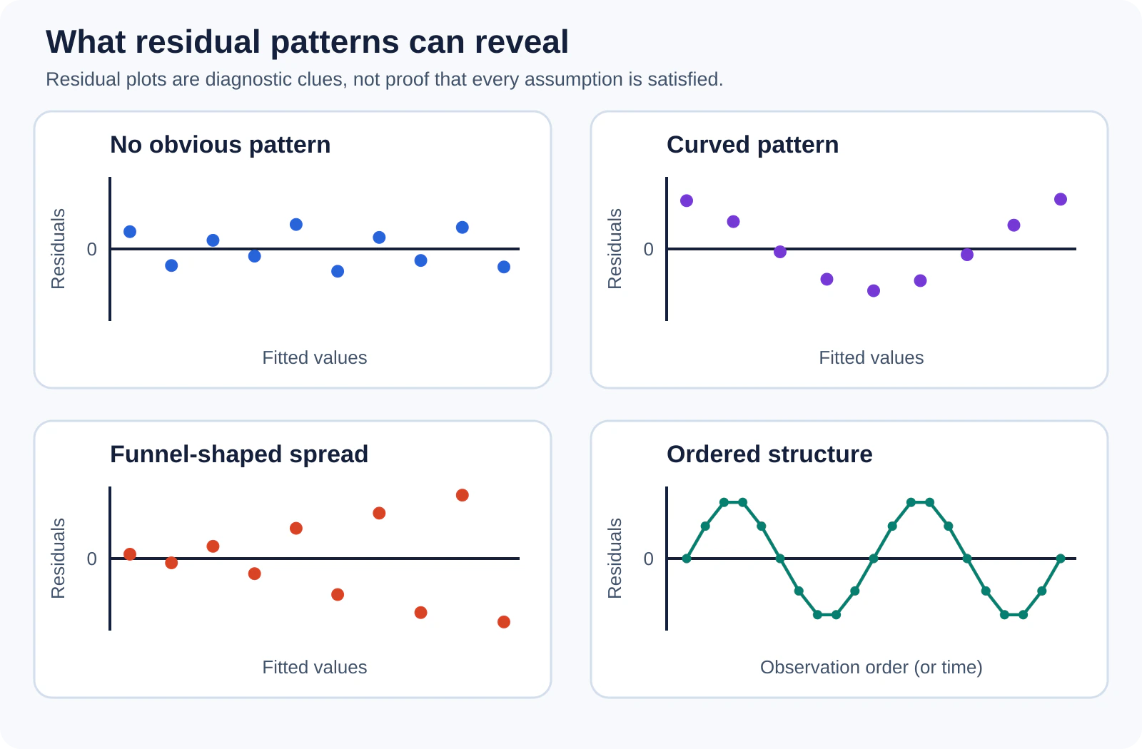
- Inspect residuals and diagnostics. Look for curves, funnels, order patterns, and influential observations.
- Use the finalized model carefully. Monitor whether new data resemble the population and range used for development.
Simple vs Multiple Linear Regression
| Version | Features | Geometry | Beginner example |
|---|---|---|---|
| Simple Linear Regression | One | A straight fitted line in two dimensions | Predict energy use from outdoor temperature |
| Multiple Linear Regression | Two or more | A plane or higher-dimensional surface | Predict energy use from temperature, floor area, and occupancy |
Both versions are linear in their fitted coefficients.
How to Evaluate Linear Regression
Regression models predict numbers, so “accuracy” is usually the wrong umbrella term. Evaluate the size and consequences of numerical errors with task-appropriate metrics. Google’s Machine Learning Crash Course explains that squared errors give large misses more weight and that MAE and RMSE stay in the target’s units. Review Google’s regression loss guide.
| Metric | What it communicates | Important nuance |
|---|---|---|
| MAE | Average absolute prediction error | Easy to interpret in the target’s units and less dominated by large errors than squared metrics |
| MSE | Average squared prediction error | Penalizes large errors more strongly; measured in squared target units |
| RMSE | Square root of MSE | Returns error to the target’s units while retaining sensitivity to large errors |
| R² | Fit relative to a baseline that predicts the mean target | 1 is best, 0 matches that baseline, and R² can be negative |
No single metric is universally best. Choose metrics based on the task and the cost of different errors. Scikit-learn documents that R² may be negative when a model performs worse than the mean-prediction baseline. See the scikit-learn R² reference. For broader metric selection, continue to Model Evaluation Metrics Explained.
Training objective is not the same as the reporting metric. OLS fits coefficients using squared residuals, but you can evaluate the resulting model with MAE, RMSE, R², or another metric that reflects the real decision.
When Is Linear Regression Appropriate?
Linear Regression is worth considering when the target is numerical, a linear approximation is plausible or useful as a baseline, and a compact coefficient-based model suits the task. Its assumptions should be interpreted in context:
- Linearity: the expected target should be reasonably represented by a linear combination of the included features.
- Independent errors: residuals should not show dependence that conflicts with the modeling setup, such as an ignored time-order pattern.
- Roughly constant variance: residual spread should not systematically widen or narrow across fitted values.
- Residual normality: this is mainly important for certain classical confidence intervals and significance tests; it is not a universal requirement for producing predictions.
Residual plots help check these conditions. Strong curves can suggest missing nonlinear structure; funnels can suggest changing variance; order patterns can suggest dependence. These signals call for investigation, not an automatic pass/fail rule.
Common Problems
Multicollinearity
If predictors contain very similar information, the model may still predict reasonably well while individual coefficient estimates become unstable or difficult to interpret.
Extrapolation
Predictions far outside the feature ranges represented by the training data are extrapolations. They may be unreliable even when the fitted model looks good inside the observed range.
Outliers and influential observations
Squared-error fitting can give unusual observations substantial weight. Investigate data quality, leverage, and domain context; do not automatically delete a point merely because it is unusual.
Underfitting and overfitting
A plain linear model can underfit a strongly nonlinear relationship or omit important interactions. Overfitting becomes more plausible as predictors, interactions, polynomial terms, and other complexity are added. See Overfitting vs Underfitting.
Penn State groups multicollinearity, extrapolation, nonconstant variance, autocorrelation, and overfitting among important regression pitfalls. Explore Penn State’s regression pitfalls lesson.
Common Extensions
- Polynomial features such as x² can let a linear model represent curvature while remaining linear in its fitted coefficients.
- Ridge Regression adds a penalty that shrinks coefficients and can improve stability when predictors are correlated.
- Lasso adds a different penalty that can shrink some coefficients to zero.
Ridge and Lasso are regularized linear models, not replacements for careful validation or diagnostics. Scikit-learn’s linear-model guide explains their objectives and trade-offs.
Strengths and Trade-offs
| Strengths | Trade-offs |
|---|---|
| Fast, compact, and useful as a baseline | Nonlinearities and interactions require explicit representation |
| Predictions can be traced to feature values and coefficients | Interpretation weakens with correlation or complex transformations |
| Introduces fitting, residuals, and evaluation clearly | Squared-error fitting is sensitive to influential observations |
| Can work well when a linear approximation suits the task | Can extrapolate poorly outside the observed range |
Linear Regression vs Logistic Regression
| Question | Linear Regression | Logistic Regression |
|---|---|---|
| What does it predict? | A numerical target | A class probability used for classification |
| Typical example | Predict energy use | Estimate the probability that an email is spam |
| Output | Usually an unrestricted number | A probability between 0 and 1 for binary logistic regression |
| Core fitting idea | Often OLS for the introductory model | A logistic model with a classification-appropriate objective |
Despite the shared name, Logistic Regression is not ordinary Linear Regression applied to category numbers. It is the next lesson because it reuses coefficients and linear combinations while changing the output and fitting setup for classification.
FAQ
Is Linear Regression supervised learning?
Yes. It learns from examples containing feature values and a known numerical target.
Why is it called linear?
The prediction is linear in the fitted coefficients. Polynomial feature transformations can represent curvature while the model remains linear in those coefficients.
Does a positive coefficient prove causation?
No. It describes an estimated association in the fitted model, holding other included features constant. Causal conclusions require stronger design and assumptions.
Can R² be negative?
Yes. On evaluation data, a negative R² means the model performed worse than the baseline that always predicts the target mean.
Should I remove every outlier?
No. First check whether it is an error, a rare but valid case, or an influential observation that reveals a modeling problem. Removal needs a defensible data and domain reason.
Continue Learning
Next lesson
Logistic Regression Explained
Learn how a related coefficient-based model estimates class probabilities for classification tasks.