
Hierarchical clustering is an unsupervised method that organizes observations into a nested tree of groups. Instead of returning only one flat partition, it shows how individual observations and larger clusters join—or split—at different levels of dissimilarity.
The tree is displayed as a dendrogram. It can help you explore possible groupings, but the result depends on the features, preprocessing, dissimilarity measure, and linkage rule you choose. This method belongs to the broader family described in Unsupervised Learning Explained.
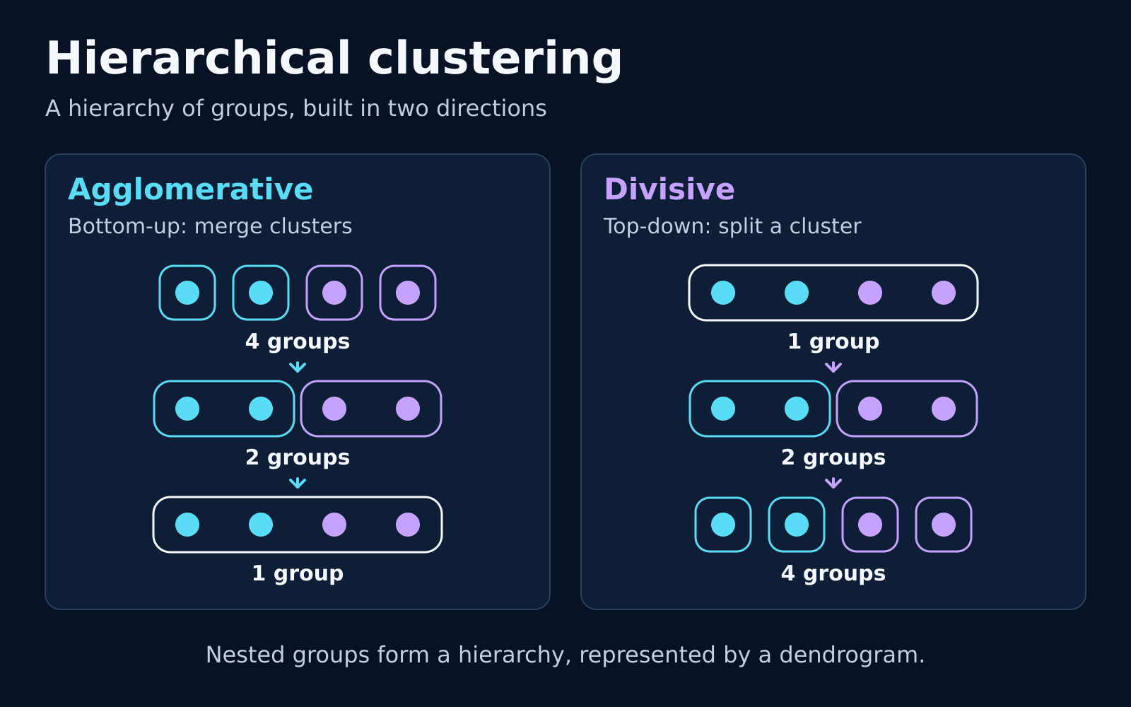
How agglomerative clustering works
The most common form is agglomerative, a bottom-up process:
Divisive hierarchical clustering works in the opposite direction: it begins with one group and recursively splits it. Divisive approaches are less common in mainstream machine-learning workflows and their computational demands depend on the particular algorithm.
A small worked example
Suppose four one-dimensional observations have the values 1, 2, 8, and 10. Using Euclidean distance and single linkage:
- Values 1 and 2 merge first because their distance is 1.
- Values 8 and 10 merge next because their distance is 2.
- The two clusters merge later because the closest cross-cluster pair—2 and 8—is 6 units apart.
A cut above 2 and below 6—for example, at 3—produces two clusters: {1, 2} and {8, 10}. A different linkage rule, scale, feature set, or outlier could change the order and the final interpretation.
How to read a dendrogram
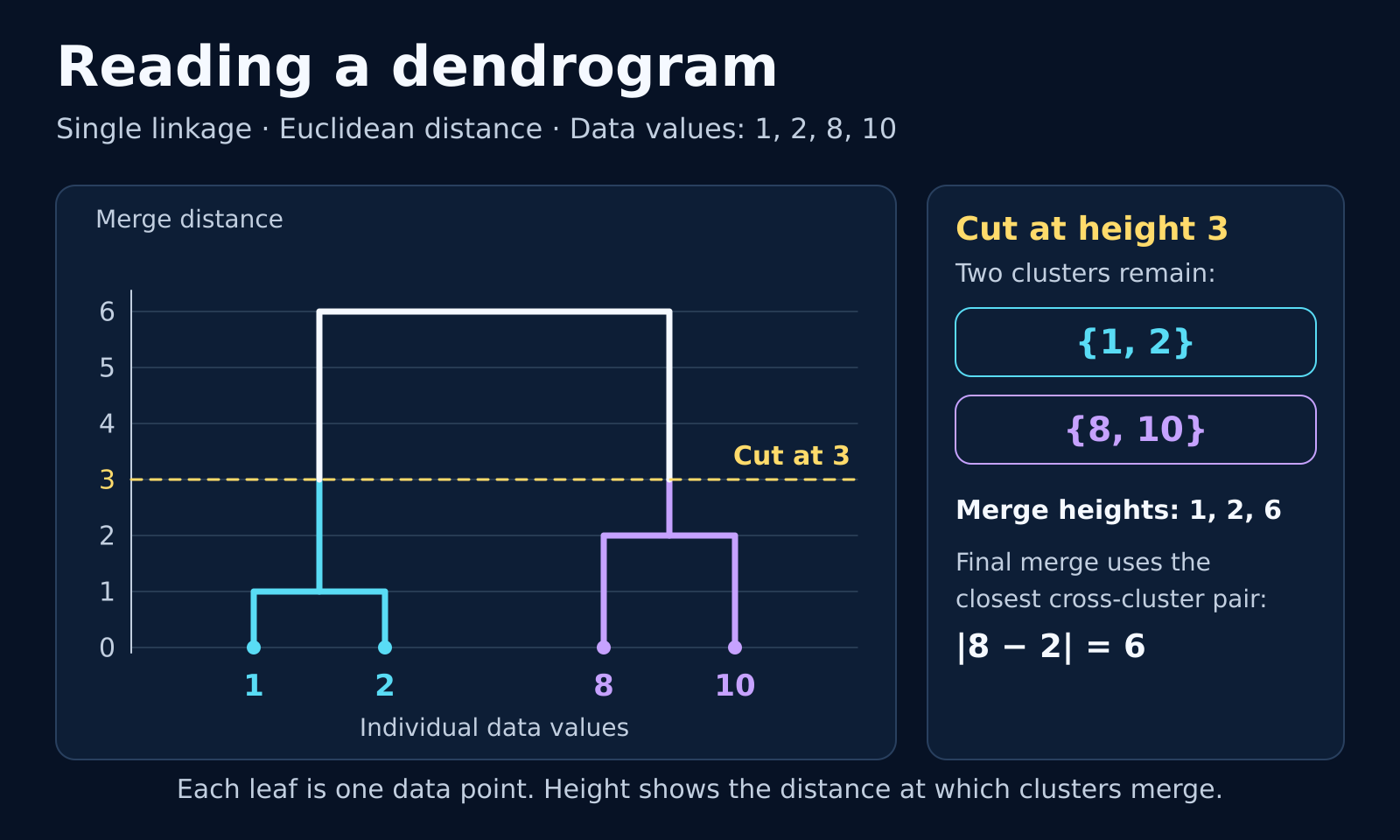
- Leaves at the bottom represent observations or already summarized groups.
- Branches record which clusters join.
- Merge height represents dissimilarity according to the chosen linkage rule.
- Horizontal order is usually arranged for display and should not be read as another measurement axis.
- A horizontal cut defines a flat clustering: every disconnected branch below the cut becomes a cluster.
A large vertical gap can suggest a useful cut, but it does not prove the correct number of clusters. Dendrograms also become crowded as the number of observations grows. The SciPy dendrogram documentation shows how a computed hierarchy is represented and visualized.
Dissimilarity measures and linkage methods
A dissimilarity measure compares observations; a linkage method defines the dissimilarity between clusters. A mathematical distance metric is one common type of dissimilarity measure. Both choices shape the hierarchy. See the SciPy linkage reference for formal linkage definitions.
Scroll horizontally to view the full comparison. Keyboard: focus this table, then use the left and right arrow keys.
| Linkage | Cluster distance | Typical behavior |
|---|---|---|
| Single | Closest pair of observations | Can recover elongated shapes but may create chains through bridge points. |
| Complete | Farthest pair of observations | Usually favors tighter groups and is sensitive to extreme pairwise distances. |
| Average | Average of cross-cluster pairwise distances | Offers a compromise between single and complete linkage. |
| Ward | Increase in total within-cluster sum of squared Euclidean distances | Often creates compact groups. Ward linkage assumes Euclidean feature-space geometry; in scikit-learn, Ward requires the Euclidean metric. |
Euclidean and Manhattan distances are common dissimilarity measures for numerical features. Cosine distance can be useful for some directional representations. The correct choice depends on what dissimilarity means for the task; measures and linkage rules are not interchangeable defaults. The scikit-learn AgglomerativeClustering reference documents its metric-linkage compatibility, including Ward’s Euclidean requirement.
Preprocessing and validation
Clustering happens in the representation you provide. With magnitude-sensitive measures such as Euclidean or Manhattan distance, a feature measured in thousands can dominate one measured between zero and one, so standardization or another justified transformation is often appropriate. Scaling is not a universal rule: the right preprocessing depends on the data type, representation, chosen dissimilarity measure, and meaning of each feature. Outliers can also change merge order substantially.
Missing values, irrelevant variables, duplicated features, arbitrary categorical codes, and high-dimensional representations can all make distance misleading. See Data Preprocessing Explained and Feature Engineering Explained.
To evaluate a proposed cut, combine several forms of evidence:
- Inspect the dendrogram and consider within-cluster cohesion and between-cluster separation.
- For a chosen flat cut, compare internal measures such as the silhouette score when its assumptions are appropriate; the score evaluates the resulting flat labels, not the hierarchy by itself.
- Check stability across samples and reasonable preprocessing choices.
- Confirm that the groups are interpretable and useful for the intended decision.
A hierarchy is an exploratory model of the selected representation—not proof that natural or causal categories exist.
When hierarchical clustering is useful
It is a reasonable choice when you want to explore nested relationships, the dataset is small or moderate, a meaningful distance can be defined, and inspecting multiple levels of grouping is more useful than committing immediately to one K.
Possible applications include exploring gene-expression patterns, organizing numerical behavior profiles, grouping document representations, and creating preliminary customer segments. Clustering may support research or decision workflows in healthcare, security, fraud, or recommendation domains, but it is not automatically a safe detector, diagnosis, or production recommendation system.
Strengths and limitations
- Nested view: one hierarchy can be inspected at several levels.
- No initial K required: the hierarchy can be built before selecting a flat cut, although a final grouping still requires a threshold or cluster count.
- Flexible definitions: multiple distances and linkage rules are available, but different choices can produce different answers.
- Computational cost: unconstrained agglomerative clustering can require substantial time and memory as the number of observations grows because many possible relationships must be considered. A sparse connectivity constraint, such as a nearest-neighbor graph, limits eligible merges and can make some workloads more tractable, but actual scalability depends on the implementation, graph density, linkage, and data; the scikit-learn hierarchical clustering guide provides implementation context for connectivity constraints.
- Irreversible merges: standard agglomerative methods do not revisit an early merge later.
- Sensitivity: scaling, outliers, noise, and unsuitable features can distort the tree.
Hierarchical clustering versus K-Means
Scroll horizontally to view the full comparison. Keyboard: focus this table, then use the left and right arrow keys.
| Question | Hierarchical clustering | K-Means |
|---|---|---|
| Output | Nested hierarchy plus an optional flat cut | One flat partition into K clusters |
| Cluster count | Can be selected after building the hierarchy | Chosen before fitting |
| Geometry | Depends on distance and linkage | Favors compact Euclidean groups around means |
| Scale | Usually better suited to small or moderate datasets | Often more scalable for larger numerical datasets |
| Inspection | Dendrogram shows nested relationships | Centroids summarize the selected partition |
Neither method is universally better. Choose according to the data, geometry, scale, and purpose. Read K-Means Clustering Explained.
Sources and further reading
- scikit-learn: Hierarchical clustering
- scikit-learn: AgglomerativeClustering
- SciPy: Hierarchical clustering
Where to learn next
Return to the machine-learning algorithm roadmap to compare this hierarchy with other clustering and prediction methods.