
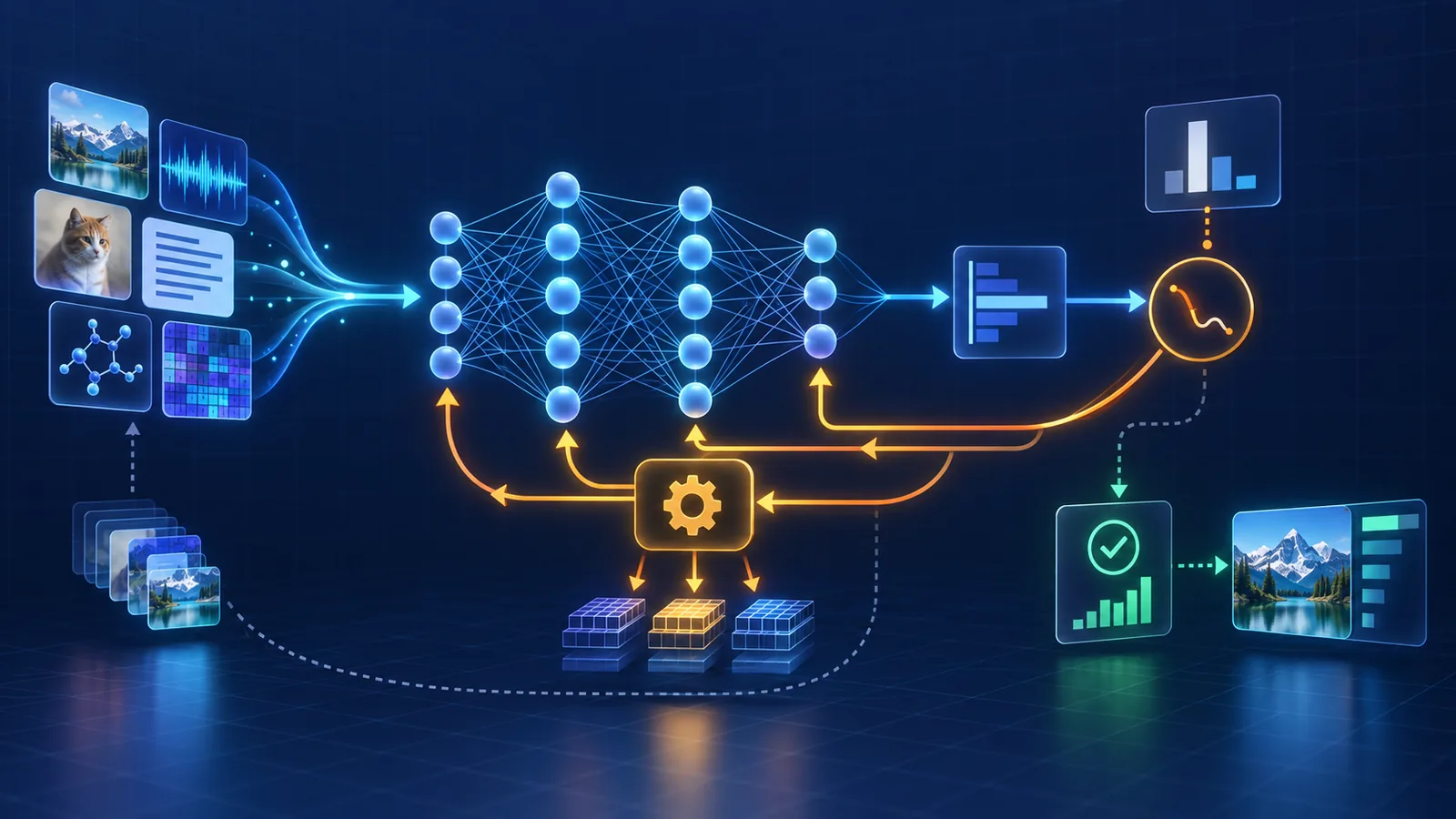
Deep learning models do not simply “get smarter” each time they see data. They are trained through a controlled loop: process a batch, measure a loss, compute gradients, update parameters, and repeat—then evaluate on data that was not used for those updates.
This beginner-friendly Lesson 9 explains that complete workflow, from the first training batch to validation, final testing, and inference. No equations are required.
Prerequisite: neural networks
A neural network contains layers and trainable parameters such as weights and biases. If those ideas are new, read the previous lesson, Neural Networks Explained, before continuing.
How deep learning works: the complete training loop
At a high level, deep learning training follows this sequence:
Load a subset of training examples.
Produce model outputs.
Score the training objective.
Compute gradients.
Update parameters using the learning rate.
Repeat: continue through batches and epochs while checking validation results and tuning development choices.
The distinction in the middle matters: backpropagation computes gradients; the optimizer uses those gradients to update parameters. PyTorch’s official training tutorial makes the same separation between loss.backward() and optimizer.step(). See PyTorch: Optimizing Model Parameters.
Step 1: Prepare data and create batches
Training begins with a dataset. Images, text, audio, video, or numerical records normally require preparation before a model can use them. Depending on the task, that can include cleaning, filtering, tokenization, resizing, normalization, encoding, sampling, augmentation, and data-quality checks.
Deep networks can learn useful internal representations and may reduce some handcrafted feature engineering, but they do not make data preparation unnecessary. More data can help when it is relevant and high quality; it does not guarantee better results.
The training set is usually divided into batches. A batch is a subset of training examples processed together. Using batches makes computation practical and provides repeated opportunities to update the model.
Step 2: Run the forward pass
During a forward pass, a batch moves through the network using the model’s current parameters. Each layer transforms the values it receives, and the last layer produces an output—for example, class scores, a predicted number, or the next-token probabilities in a language model.
Some vision networks provide an intuitive illustration: early layers may respond to edges, later layers to textures or shapes, and deeper layers to more task-specific patterns. That edge → shape → object story is illustrative, not a universal rule for every vision model, transformer, language model, or multimodal system.
Step 3: Calculate the loss or objective
A loss function produces a numerical signal describing how well the model is meeting its training objective. In a supervised cat-versus-dog example, the loss compares the model’s output with the known label. Other systems can use self-supervised, reconstruction, generative, or reinforcement-learning objectives, so a loss is broader than simply “the difference from the correct answer.”
Training aims to improve the chosen objective, but the loss will not necessarily decrease on every batch. Training can be noisy, plateau, become unstable, converge poorly, or fail.
Step 4: Backpropagation computes gradients
Backpropagation calculates how the loss changes with respect to each trainable parameter. Those calculated changes are called gradients. A gradient tells the training system how a small change to a parameter would affect the loss.
Backpropagation does not perform the parameter update by itself. It supplies the information that the optimizer needs for the next stage.
Step 5: The optimizer updates parameters
An optimizer uses the gradients to update weights, biases, and other trainable parameters. Gradient descent is the basic idea of changing parameters in a direction intended to reduce the loss. Stochastic gradient descent (SGD) and Adam are common optimizer examples.
The learning rate controls the size of the updates. A rate that is too large can make training unstable or skip useful solutions. A rate that is too small can make progress very slow. The best choice depends on the model, data, optimizer, and training setup.
It is misleading to say “useful patterns get stronger weights” and “irrelevant patterns get weaker weights.” Individual parameter sizes do not map neatly to human-readable usefulness. More accurately, the optimizer adjusts many interacting parameters in ways intended to improve the training objective.
Step 6: Repeat through batches and epochs
- Batch: a subset of training examples processed together.
- Training step or iteration: one parameter-update step, commonly based on one batch.
- Epoch: one complete pass through the training dataset.
After an update, the model processes another batch. The loop continues across many batches and often several epochs. The goal is not merely to minimize training loss. It is to learn patterns that work on relevant, unseen data.
Step 7: Validate and tune without using the final test
A sound development workflow gives different jobs to three data partitions:
- Training data is used to calculate training losses and update parameters.
- Validation data is checked during development to compare choices, tune hyperparameters such as learning rate, monitor generalization, and support decisions such as early stopping.
- Test data is held back for final evaluation after development decisions are complete.
The important pattern is train ↔ validate and tune → final test. Repeatedly changing the model because of test results leaks information from the test set into development and makes that final score less trustworthy. Google’s Machine Learning Crash Course likewise recommends training, validation, and test sets, with the test set used for the final check. See Google: Dividing the original dataset.
Generalization, overfitting, and early stopping
Generalization means performing usefully on relevant examples the model did not train on. A model can reduce its training loss while its validation performance stops improving or gets worse. That gap is a warning sign of overfitting: the model fits the training data too closely and performs poorly on new data.
Common controls include regularization techniques such as dropout, weight decay, and data augmentation. Early stopping ends training according to a defined criterion when validation performance stops improving. These methods can help, but none guarantees good generalization. Learn more in Overfitting vs Underfitting, and see Google’s overview of overfitting and generalization.
Final test and inference
Once model and tuning decisions are finished, the held-back test set provides a final estimate of performance on unseen examples. A good test result is evidence about that test setup—not a guarantee of perfect real-world performance. Real data can differ or change over time.
Inference is what happens after training when the model uses its learned parameters to produce an output for new input. During ordinary inference, the model is not running backpropagation or updating its parameters. A deployed model therefore does not automatically learn from every interaction unless a separate training or adaptation system has been designed to do so.
How architectures fit into the same process
Convolutional neural networks, recurrent neural networks, and transformers use different structures and are suited to different kinds of problems. Many are still trained through the same broad pattern: forward computation, a loss or objective, gradient calculation, and optimization. Architecture details belong in their dedicated guides; this lesson owns the training mechanics.
Artificial neural networks were historically inspired in part by biological neurons, but modern deep-learning systems are mathematical computational models. They do not learn, reason, or understand in the same way humans do.
A compact example: training an image classifier
- Prepare labeled cat and dog images, then split them into training, validation, and test sets.
- Send one training batch through the network in a forward pass.
- Use a loss function to score the outputs against the batch labels.
- Run backpropagation to compute gradients.
- Let the optimizer update the parameters using the selected learning rate.
- Repeat for more batches and epochs, monitoring validation results and adjusting development choices.
- After tuning is complete, evaluate once on the held-back test set.
- Use the trained model for inference on new images without ordinary training updates.
Frequently asked questions
What is backpropagation in simple terms?
Backpropagation computes gradients: information about how the loss changes with each trainable parameter. The optimizer—not backpropagation itself—uses those gradients to update the parameters.
What is the difference between a batch and an epoch?
A batch is a subset of training examples processed together. An epoch is one full pass through the entire training dataset, usually made up of many batches.
Does training improve a model on every step?
No. Results can fluctuate, plateau, become unstable, or improve on training data while worsening on validation data. Training is monitored because improvement is not guaranteed.
Does deep learning always require labeled data?
No. Supervised learning uses labels, while self-supervised and other objectives can learn from different signals. The broad forward pass, objective, backpropagation, and optimization pattern still applies to many systems.
Does a deployed model learn from every interaction?
Usually not. Ordinary inference produces outputs with fixed learned parameters. Updating a deployed model requires a separate training, fine-tuning, or online-learning process.
Key takeaway
Deep learning training is a sequence of distinct operations: batch → forward pass → loss or objective → backpropagation computes gradients → optimizer updates parameters using a learning rate → repeat through batches and epochs → validate and tune → final test → inference.
The training loop tries to improve an objective; validation helps guide development; the held-back test checks the finished model; and inference uses the trained model without ordinary parameter updates.
Next lesson: Dataset Fundamentals
Now that you understand the training loop, learn what training examples are made of and why data quality matters: What Is a Dataset in Machine Learning?
Previous lesson: Neural Networks Explained. Related depth: Deep Learning vs Machine Learning.