
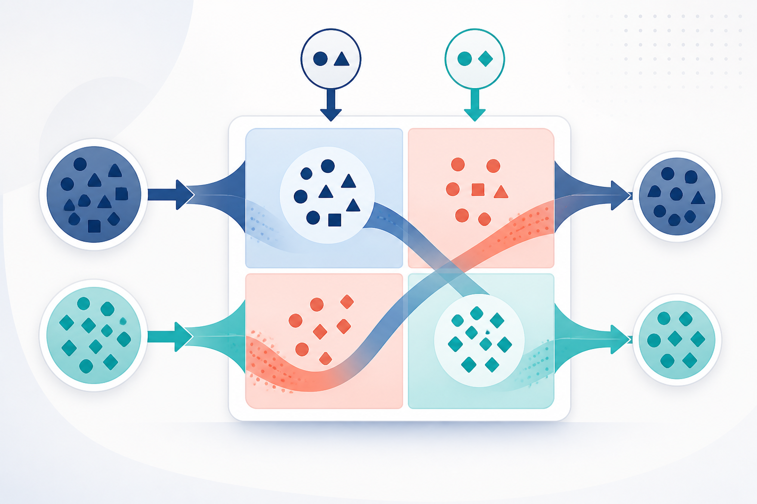
A confusion matrix shows exactly where a classification model is right and where it is wrong. Instead of reporting one overall score, it separates correct predictions from the two kinds of mistakes a model can make.
Updated:
This guide uses one consistent spam-filter example to explain true positives, true negatives, false positives, and false negatives. You will also learn how to calculate the most common evaluation metrics, how decision thresholds affect the matrix, and how to read multiclass and normalized matrices.
What is a confusion matrix?
A confusion matrix is a table that compares a classifier’s predicted labels with the labels that were actually observed. For binary classification, the table has four cells:
- True positive (TP): the model predicts the positive class, and the example is actually positive.
- True negative (TN): the model predicts the negative class, and the example is actually negative.
- False positive (FP): the model predicts the positive class, but the example is actually negative.
- False negative (FN): the model predicts the negative class, but the example is actually positive.
“Positive” does not automatically mean good, and “negative” does not automatically mean bad. They are simply the two class labels. In a spam filter, we can define spam as the positive class and not spam as the negative class.
A complete spam-filter example
Suppose we test a spam filter on 100 emails. Fifty are actually spam and 50 are legitimate. The model produces these results:
On a phone: swipe horizontally to view every column in the matrix.
| Actual class | Predicted spam | Predicted not spam | Row total |
|---|---|---|---|
| Actual spam | 40 True positives | 10 False negatives | 50 |
| Actually not spam | 5 False positives | 45 True negatives | 50 |
| Column total | 45 | 55 | 100 |
The model correctly identifies 40 spam emails and correctly leaves 45 legitimate emails alone. It incorrectly flags five legitimate emails as spam and misses 10 spam emails.
Metrics calculated from the matrix
The four counts support several complementary metrics. No single metric tells the whole story.
Accuracy
Accuracy is the share of all predictions that are correct.
Accuracy = (TP + TN) / (TP + TN + FP + FN) = (40 + 45) / 100 = 85%
Accuracy is easy to understand, but it can be misleading when one class is much more common than the other.
Precision
Precision asks: of the emails predicted as spam, how many were actually spam?
Precision = TP / (TP + FP) = 40 / 45 = 88.9%
Higher precision means fewer legitimate emails are incorrectly sent to spam.
Recall (sensitivity)
Recall asks: of all the emails that were actually spam, how many did the model catch?
Recall = TP / (TP + FN) = 40 / 50 = 80%
Higher recall means fewer spam emails reach the inbox.
Specificity
Specificity asks: of all legitimate emails, how many did the model correctly leave out of spam?
Specificity = TN / (TN + FP) = 45 / 50 = 90%
F1 score
The F1 score is the harmonic mean of precision and recall. It is useful when you want one number that penalizes a large imbalance between those two metrics.
F1 = 2 × (precision × recall) / (precision + recall) ≈ 84.2%
F1 does not include true negatives, so it is not automatically the best choice for every problem. Choose metrics according to the real cost of each kind of error.
Why accuracy can hide a weak model
Imagine a dataset in which 95% of emails are legitimate and only 5% are spam. A model that predicts “not spam” for every email would be 95% accurate, but it would catch none of the spam. Its recall for spam would be 0%.
The confusion matrix exposes that failure because every spam email appears in the false-negative cell. Accuracy is not “worse” than a confusion matrix; it is one summary calculated from it. The matrix provides the detail needed to interpret that summary.
Decision thresholds change the matrix
Many classifiers first produce a probability or score. A decision threshold converts that score into a class label. For example, a spam filter might classify an email as spam when its predicted spam probability is at least 0.50.
- Lowering the threshold usually catches more positives, increasing recall, but it can also create more false positives and reduce precision.
- Raising the threshold usually reduces false positives, but it can create more false negatives and lower recall.
There is no universally correct threshold. The appropriate tradeoff depends on the application, the costs of errors, class prevalence, and how the model will be used. Evaluate thresholds on validation data, then report final performance on untouched test data.
Raw counts vs normalized confusion matrices
A raw confusion matrix shows counts, such as 40 true positives. A normalized matrix converts counts to proportions or percentages. Normalization can make class-level performance easier to compare when classes have very different sizes.
- Normalize by actual class (row): each row sums to 100%. This highlights recall for each class.
- Normalize by predicted class (column): each column sums to 100%. This highlights how reliable each predicted label is.
- Normalize across the full matrix: all cells sum to 100%. This shows each cell’s share of the entire dataset.
Always state the normalization method and confirm which axis represents actual labels. Libraries do not all display matrices in the same orientation.
How to read a multiclass confusion matrix
A multiclass classifier has more than two labels, so the matrix expands to one row and one column per class. Correct predictions appear on the main diagonal. Off-diagonal cells show which pairs of classes the model confuses.
For example, an image classifier might distinguish cats, dogs, and rabbits. A large cell at “actual rabbit, predicted cat” identifies a specific error pattern that an overall accuracy score cannot reveal.
You can calculate precision, recall, and F1 for each class by treating that class as positive and all other classes as negative. To summarize across classes, common averaging methods include:
- Macro average: gives every class equal weight.
- Weighted average: weights each class by the number of examples it contains.
- Micro average: aggregates decisions across all classes before calculating the metric.
When classes are imbalanced, report per-class results alongside an appropriate average. A strong result for a common class can otherwise hide weak performance on a rare one.
Error names and real-world costs
In classical hypothesis testing, a false positive can correspond to a Type I error and a false negative to a Type II error—but only after the positive class and null hypothesis have been defined consistently. In machine learning, the plain terms “false positive” and “false negative” are usually clearer.
The more important question is what each error costs in the actual system. In a spam filter, a false positive may hide an important legitimate message, while a false negative may allow unwanted mail into the inbox. In another application, the balance can be very different.
For healthcare, hiring, lending, safety, or other high-impact decisions, a confusion matrix is only one part of evaluation. Teams should also examine subgroup performance, calibration, data quality, distribution shifts, uncertainty, human oversight, and the consequences of errors. A favorable matrix alone does not establish that a system is fair, safe, or suitable for deployment.
A practical interpretation checklist
- Confirm which label is the positive class.
- Check whether rows are actual labels or predicted labels.
- Inspect the raw counts before relying on percentages.
- Consider class imbalance and the data’s real-world prevalence.
- Calculate the metrics that match the application’s error costs.
- Test how performance changes across reasonable decision thresholds.
- For multiclass problems, inspect every class and the largest off-diagonal errors.
- Evaluate on data that was not used to train the model.
Frequently asked questions
Is a confusion matrix only for binary classification?
No. It works for binary and multiclass classification. A multiclass matrix adds one row and one column for every class.
What makes a confusion matrix “good”?
There is no universal pattern that is good in every setting. More correct predictions and fewer errors are generally desirable, but the importance of each cell depends on class balance, thresholds, and the real consequences of false positives and false negatives.
Can a confusion matrix be used for regression?
Not directly. Confusion matrices evaluate discrete class labels. Regression models predict continuous values and typically use metrics such as mean absolute error, mean squared error, or R-squared.
Sources and further reading
- Google Machine Learning Crash Course: Accuracy, precision, recall, and related metrics
- scikit-learn documentation: Confusion matrix
What to learn next
Primary next lesson: now that you can organize classification outcomes, compare how accuracy, precision, and recall emphasize different kinds of success and failure.
Need the broader framework? Return to the Model Evaluation Metrics overview. If classification and regression are still new, review Classification vs Regression.