
Quick answer: Gradient descent is an optimization method that adjusts a model’s parameters using the slope of its loss function. It takes a step opposite the gradient, with a learning rate controlling the scale of the update. It is a training method, not a model, and reducing training loss does not prove that predictions will work well on new data.
If you have read Machine Learning Explained, you have seen the idea of learning from examples. This guide opens up one adjustment. You will calculate a prediction, measure its error, change one parameter and check what happened.
What does gradient descent change?
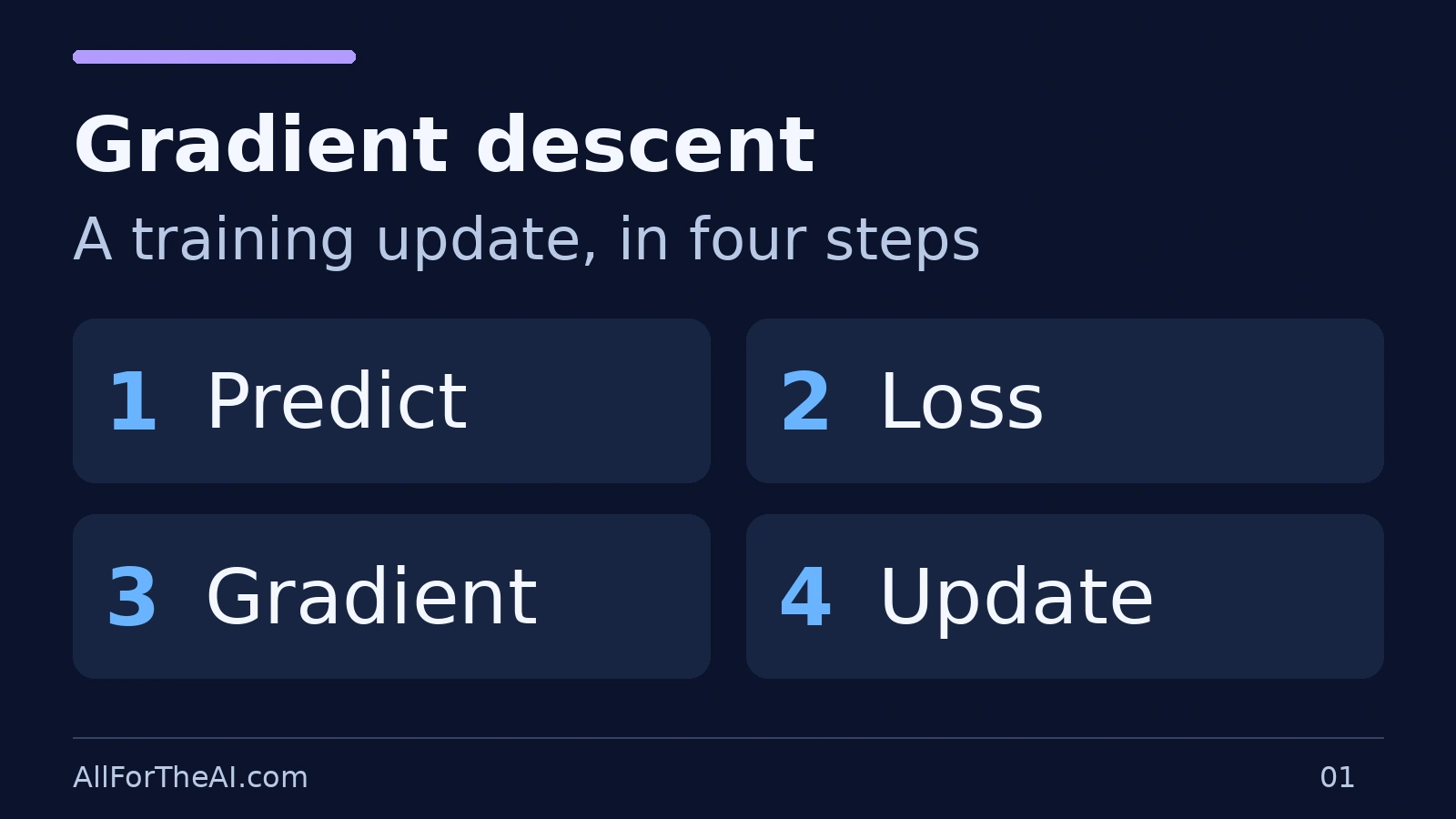
A parameter is a number inside a model that training can adjust. A loss function measures how well the current predictions match the training objective. The gradient describes how that loss changes as the parameters change.
For one parameter, the gradient is simply a derivative: a local slope. With many parameters, it is a collection of partial derivatives. Basic gradient descent uses:
new parameter = old parameter − learning rate × gradient
The minus sign matters. A positive gradient leads to a smaller parameter; a negative gradient leads to a larger one. This is local guidance, not a map revealing the best solution in advance. Google’s gradient-descent lesson introduces this loss-minimizing process.
A downhill sketch is useful, but read its axes correctly: one axis represents a parameter value and another represents loss. It is not a graph of a model’s intelligence.
A tiny worked example
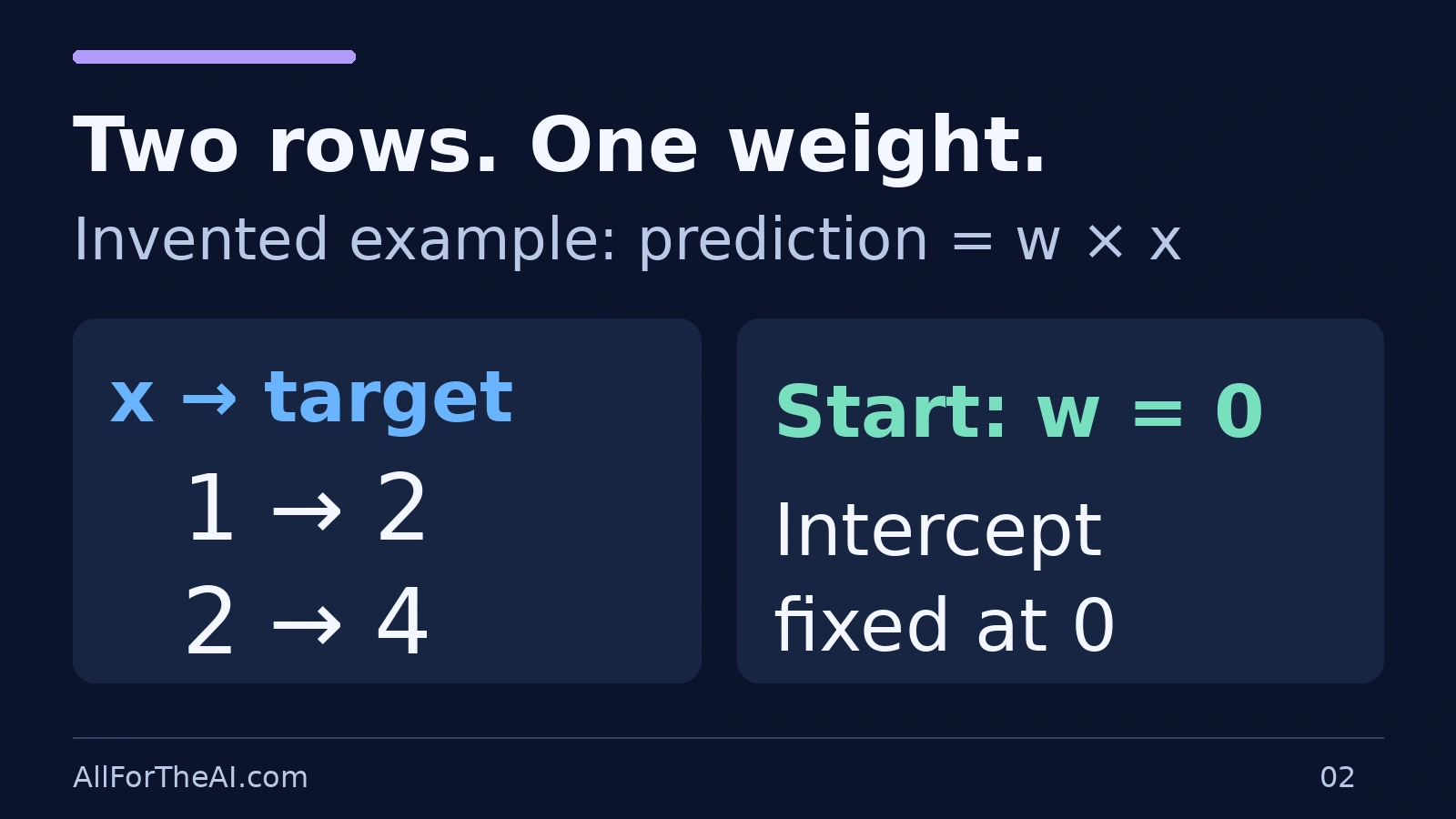
We will use an intentionally small, invented dataset:
| Input x | Target y |
|---|---|
| 1 | 2 |
| 2 | 4 |
Our model predicts y-hat = w × x. We hold the intercept at zero so there is only one adjustable number, w. This is a teaching example, not a realistic validation study or a recommended model for real-world use.
The two examples happen to follow y = 2x exactly. That lets us check the arithmetic against an obvious answer: w = 2. The training procedure below still starts at w = 0 and calculates its updates.
For a broader introduction to model form, see Linear Regression Explained.
1. Predict with the starting weight
At w = 0, both predictions are zero.
| Input | Target | Prediction | Prediction − target | Squared error |
|---|---|---|---|---|
| 1 | 2 | 0 | −2 | 4 |
| 2 | 4 | 0 | −4 | 16 |
We define our loss as the mean squared error, without an additional one-half factor:
L(w) = [(w − 2)² + (2w − 4)²] / 2
At w = 0, the loss is (4 + 16) / 2 = 10.
The definition matters. A different constant factor in the loss changes the gradient’s scale, even when the best-fitting weight stays the same.
2. Calculate the gradient
Think of the gradient as a direction check: if it is negative, increasing the weight a little lowers the loss; if it is positive, decreasing the weight a little lowers the loss. You do not need calculus to follow the next steps: use the supplied formula, then check what the update does.
For this particular loss, expanding and differentiating gives:
L(w) = 2.5(w − 2)²
gradient = dL/dw = 5(w − 2)
At w = 0, the gradient is −10. Increasing w slightly will reduce the loss locally. If calculus is new, use the supplied gradient formula for now: substitute the current weight and calculate.
Notice that the gradient is not the same as either prediction error. It summarizes how changing this shared weight affects the loss over both examples.
3. Apply one update
Try it yourself before looking at the worked step below: starting at w = 0, with gradient −10 and learning rate 0.1, should the weight increase or decrease? What new weight do you get?
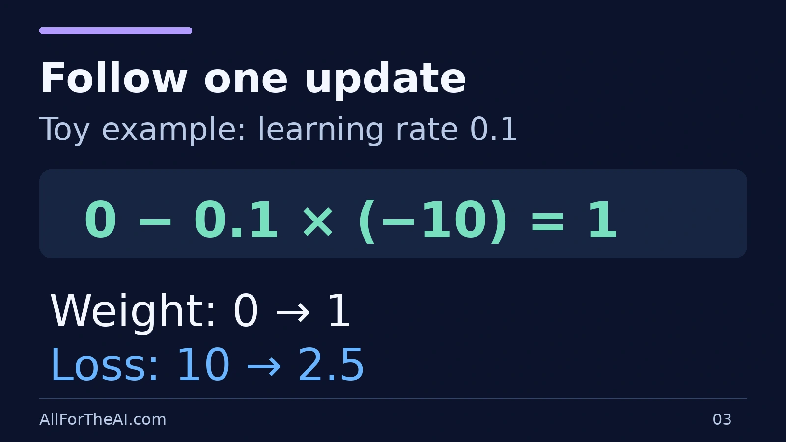
Choose a learning rate of 0.1 for this example.
new w = 0 − 0.1 × (−10) = 1
The updated weight is 1, not 0.1. The learning rate multiplies the gradient; it is not itself the amount added to every parameter.
4. Recalculate, rather than assume improvement
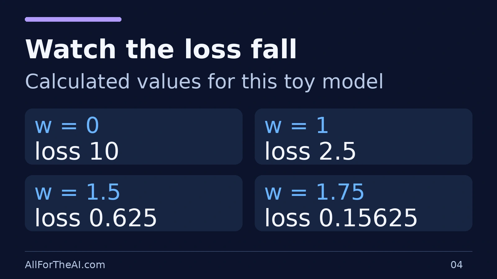
At w = 1, predictions are 1 and 2. Squared errors are 1 and 4.
new loss = (1 + 4) / 2 = 2.5
The loss fell from 10 to 2.5. Repeat the calculation with the new weight, not the old gradient:
| Completed updates | Weight | Loss |
|---|---|---|
| 0 | 0 | 10 |
| 1 | 1 | 2.5 |
| 2 | 1.5 | 0.625 |
| 3 | 1.75 | 0.15625 |
These are calculated results for this toy problem. They are not benchmark measurements. The loss reaches zero at w = 2 because the invented points fit the restricted model exactly. Most real datasets do not behave this neatly.
Why the learning rate matters
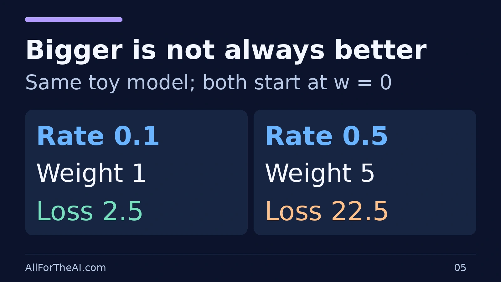
The learning rate scales the change to the parameters. Too small can mean slow progress; too large can make training unstable. There is no single best value for every model and dataset. Batch size and training duration are separate settings. Google’s hyperparameter guide explains these distinctions.
Our tiny example makes the difference visible. Start at w = 0 each time and perform just one update:
| Learning rate | New weight | New loss | What happened here |
|---|---|---|---|
| 0.01 | 0.1 | 9.025 | Small improvement |
| 0.1 | 1 | 2.5 | Larger improvement |
| 0.4 | 4 | 10 | Crossed the minimum without lowering loss |
| 0.5 | 5 | 22.5 | Loss increased |
With 0.4, the next weight returns to 0: this exact example oscillates between 0 and 4. With 0.5, the next weight is −2.5 and the loss grows again. Crossing the minimum is not automatically failure, but an oversized step can prevent convergence.
These rates illustrate the chosen equation only. They are not settings to copy into an unrelated training job.
Full-batch, stochastic and mini-batch updates
The example above uses both training rows for every gradient. That is a full-batch update.
A stochastic update can use one sampled example. A mini-batch update uses a subset. Different subsets can produce different gradients, so the loss need not fall smoothly after every update. In everyday usage, “SGD” sometimes includes mini-batch training, so check the stated batch size rather than relying on the name alone.
SGD is an optimization technique, not a model family. It can fit different models and objectives. Feature scaling can also affect its behavior; learned scaling should be fitted on training data, not held-out data. Scikit-learn’s SGD documentation explains both points.
Gradient descent is not backpropagation
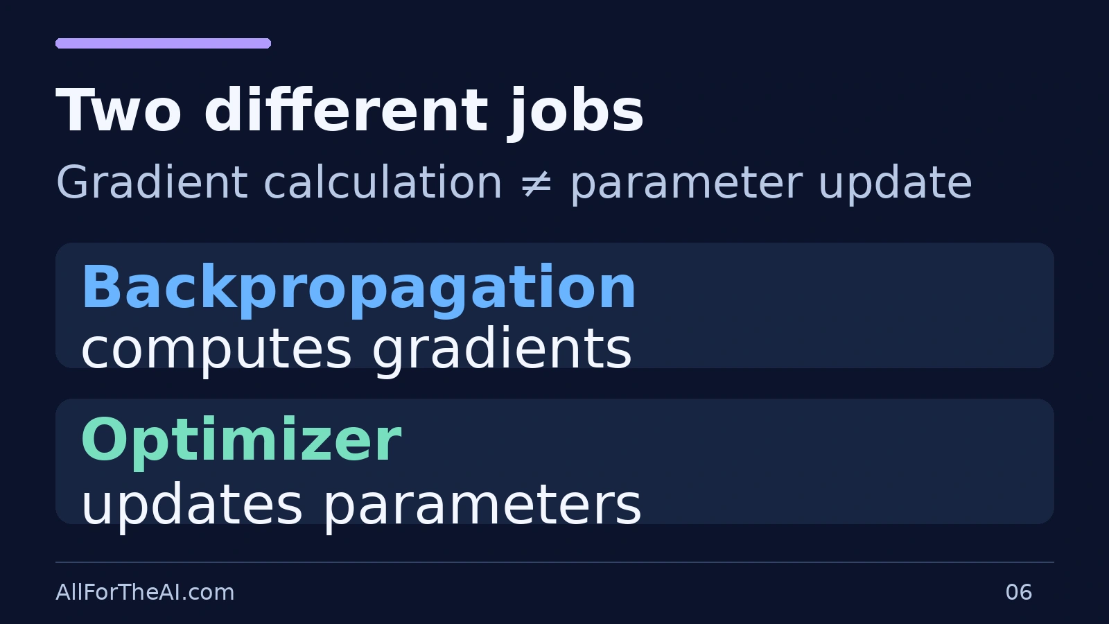
In a neural network, backpropagation computes gradients through the network. An optimizer then uses those gradients to change parameters. Those are different jobs.
PyTorch’s training example separates the backward calculation from the optimizer update. It also clears accumulated gradients between ordinary training iterations. PyTorch: Optimizing Model Parameters.
For the complete surrounding loop, continue to How Deep Learning Works. The one-weight calculation here is meant to explain the update, not replace a neural-network training guide.
What lower loss does not tell you
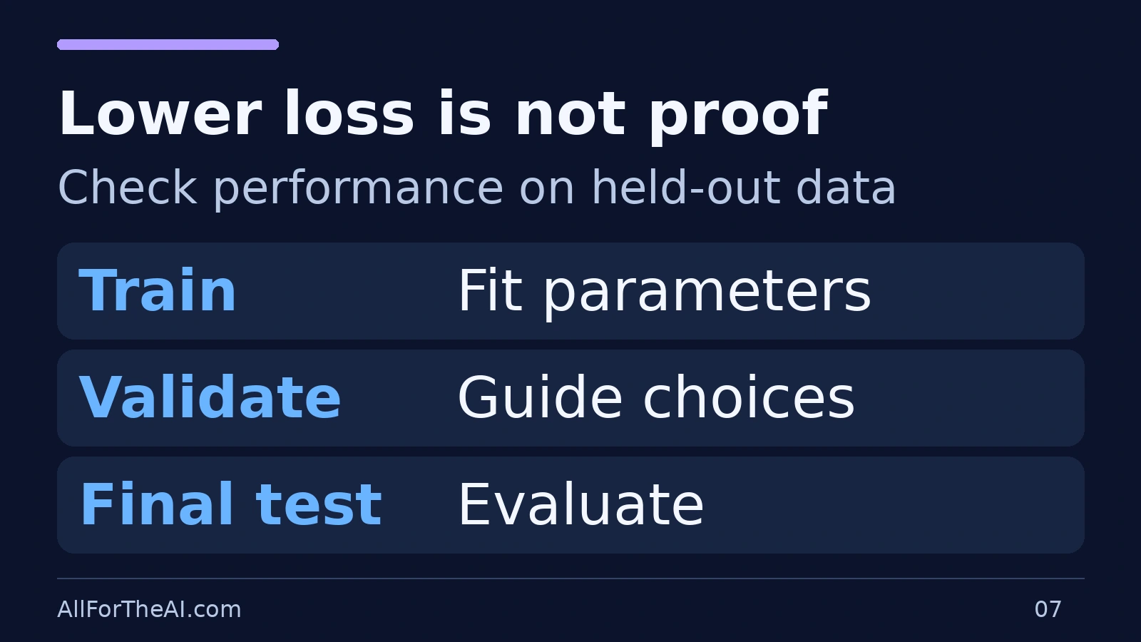
Optimization is only part of learning. A model may reduce its training objective without becoming more useful on unseen examples. Neural-network optimization also need not behave like a simple one-dimensional bowl; flat regions, saddle points and other complications matter. A global best solution is not guaranteed in general. Deep Learning, chapter 8.
Check development choices with validation data and reserve the final test for evaluation. See Training vs Testing Data and Overfitting vs Underfitting.
Nor does ordinary inference require this training update. Producing a prediction and adjusting learned parameters are distinct operations. Training vs Inference walks through that boundary.
Try one step yourself
Use the same loss and gradient. Start at w = 3, with learning rate 0.1.
- Is the gradient positive or negative?
- Will the update increase or decrease the weight?
- What are the new weight and loss?
Answer: The gradient is 5(3 − 2) = 5, so the update decreases the weight. The new weight is 3 − 0.1 × 5 = 2.5. Its loss is 2.5(2.5 − 2)² = 0.625, down from 2.5.
The lesson is not “always increase the weight.” It is “calculate the slope at the current weight, then move in the opposite direction.”
Key takeaway
Gradient descent connects a measured loss to a parameter update. Ask four questions: What is being adjusted? What loss is being minimized? Which gradient is being used? How large is the learning-rate-scaled step? Then check held-out performance separately.
Frequently asked questions
Is gradient descent a machine-learning model?
No. It is an optimization method used to adjust parameters. A model specifies how inputs become predictions; the optimizer specifies how adjustable parameters are updated.
What is a gradient?
It is the collection of derivatives of a function with respect to its parameters. For our one-weight example, it is the slope of loss with respect to that weight.
Why subtract the gradient?
The gradient points locally toward increasing loss. Subtracting a suitably scaled gradient moves in the opposite direction; a large finite step can still raise loss.
Is the learning rate the size of the update?
Not by itself. In basic gradient descent, the update is the learning rate multiplied by the gradient. Different gradients produce different changes at the same learning rate.
Does every update reduce loss?
No. An overly large step can increase loss, and sampled-batch gradients introduce variability. The smooth toy sequence is not a promise about every training run.
Does gradient descent always find the global minimum?
No. Guarantees depend on the objective and algorithm conditions. The simple quadratic example does not represent every neural-network loss landscape.
Is gradient descent the same as backpropagation?
No. Backpropagation computes gradients; the optimizer uses them to update parameters.
Does lower training loss prove better predictions?
No. Evaluate on appropriate held-out data. A lower training loss can coexist with poor generalization.
Where to Learn Next
Recommended next lesson: Continue with How Deep Learning Works to see how this parameter update fits into the wider neural-network training loop.
Continue to How Deep Learning Works
- Separate fitting from evaluation: Training vs Testing Data.
- Understand why lower training loss is not enough: Overfitting vs Underfitting.