
An imbalanced dataset contains classes that appear at very different frequencies. In classification, that can let a model look accurate while missing the cases you care about most.
If only 1% of transactions are fraudulent, predicting “not fraud” every time gives 99% accuracy and catches no fraud. A useful response starts with the cost of mistakes, meaningful metrics, and an honest evaluation. Making every class the same size is not the goal.
This guide explains how to evaluate uneven classes, compare training strategies, and avoid a common source of misleading results: resampling data before the split.
Majority and minority classes
In a binary classification problem, the majority class has more examples and the minority class has fewer. A dataset with 9,900 legitimate transactions and 100 fraudulent transactions has a 99% majority class and a 1% minority class. Google’s class-imbalance guide introduces these terms.
The positive class is the outcome designated as the event of interest. It is often the minority class, but those terms describe different things: the positive label identifies the target, while minority describes its frequency.
Class imbalance is not automatically a defect. Equipment failures, fraud, and manufacturing defects may genuinely be rare. What matters is whether the data represents the task and whether the model handles important outcomes well. There is no universal percentage at which a dataset becomes unusable.
Also check the number of examples, not just the ratio. A rare class may contain thousands of varied cases or only a handful. Those situations provide very different amounts of evidence.
Why 99 percent accuracy can hide failure
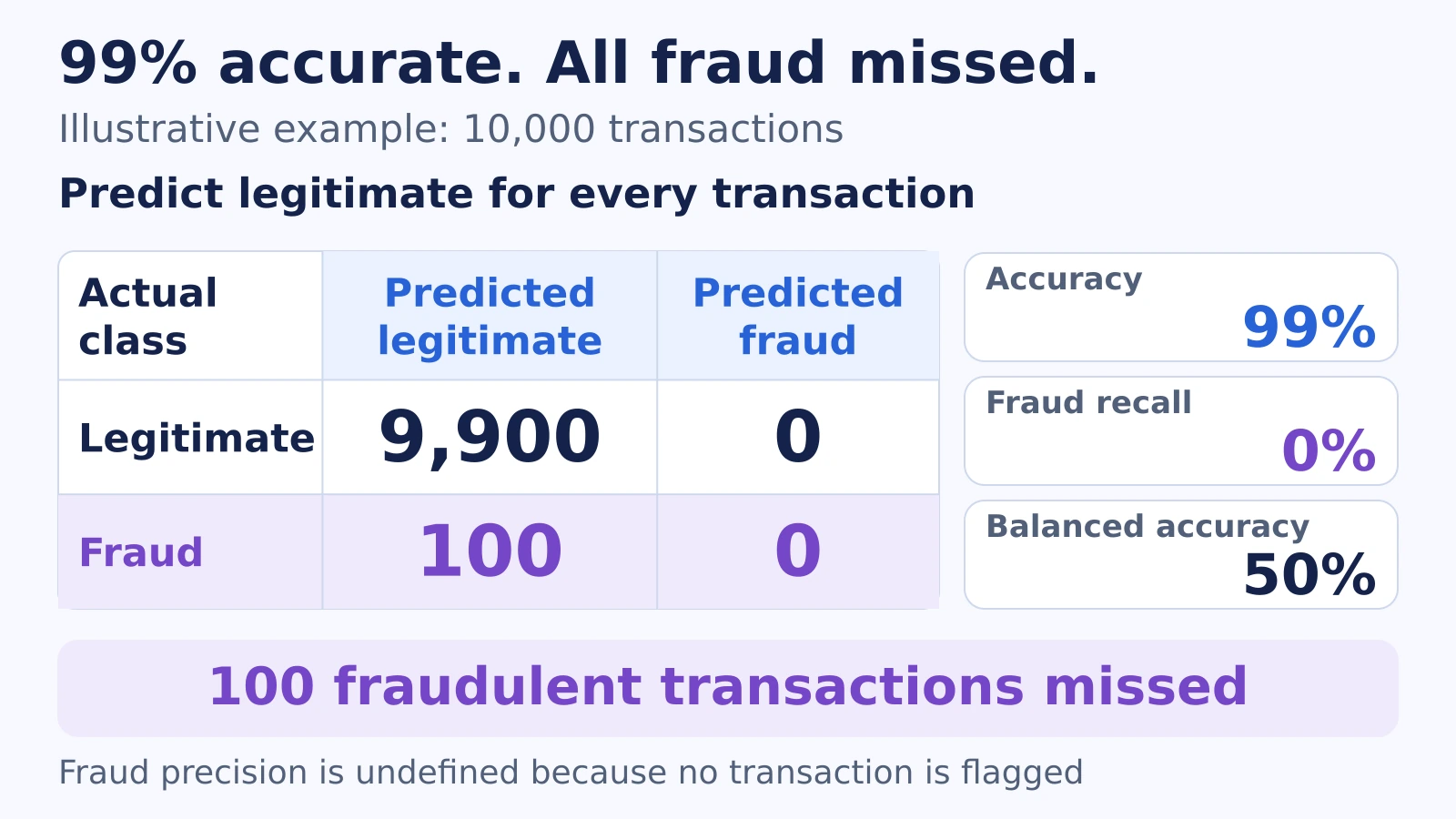
Imagine a test set of 10,000 transactions: 9,900 legitimate and 100 fraudulent. A classifier labels every transaction legitimate. This is an illustrative example, not a reported experiment.
| Actual class | Predicted legitimate | Predicted fraud |
|---|---|---|
| Legitimate | 9,900 | 0 |
| Fraud | 100 | 0 |
The model is correct on 9,900 transactions, so accuracy is 99%. It detects zero of the 100 fraudulent transactions, so fraud recall is 0%. Fraud precision is undefined because there are no predicted fraud cases; software may display a configured fallback value. Do not interpret that fallback as evidence of useful detection.
This is why a confusion matrix belongs beside the headline score. It shows which errors produced that score.
Choose metrics around the decision
Begin by asking what happens after a positive prediction and what happens when the model misses a real case. A fraud-review team may need to find more fraud while staying within its investigation capacity. Another application may place a much higher cost on false alarms.
- Precision asks how many predicted positive cases are actually positive. It helps describe the reliability of an alert.
- Recall asks how many actual positive cases were found. It exposes missed cases.
- F1 score combines precision and recall using their harmonic mean. It does not account for true negatives or encode your specific error costs.
These definitions and tradeoffs are covered in Google’s classification metrics guide. For a beginner-friendly comparison, read Accuracy vs Precision vs Recall.
Balanced accuracy
Balanced accuracy averages recall across classes, giving each class equal weight. For a binary problem, it is the average of positive-class recall and negative-class recall, also called specificity. See the scikit-learn definition.
In the transaction example, fraud recall is 0% and legitimate-transaction recall is 100%. Their average is 50%, so ordinary, unadjusted balanced accuracy is 50%. That makes the failure on one class more visible than 99% accuracy does. It still does not tell you whether the number or cost of false alarms is acceptable.
Precision and recall across thresholds
A precision–recall curve shows the tradeoff across score thresholds. It is useful when the positive class is rare, but report the positive-class prevalence alongside it: precision depends on how common positives are in the evaluated population. The scikit-learn curve reference explains its construction.
If reporting a summary, name the calculation. Average precision and trapezoidal area under a precision–recall curve are not identical. Scikit-learn’s average precision reference explains the distinction. A curve summary also does not replace precision, recall, and error counts at the threshold you will actually use.
There is no universal best metric. Choose a main measure for the decision, then report supporting measures that reveal its blind spots.
Split first and preserve realistic evaluation data
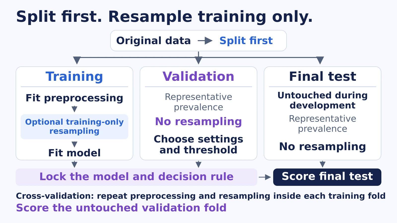
Separate the data before trying oversampling, undersampling, or synthetic sampling. Training data teaches the model. Validation data supports model, sampling, and threshold choices. Keep a final test set outside that development loop.
For independent classification examples, stratification can help preserve approximate class proportions. If records share a person, device, or other group, or the task predicts future events, use a split that respects those relationships. Stratification must not override group separation or time order. The scikit-learn cross-validation guide covers these alternatives.
Validation and test data should represent the intended deployment population, including its class prevalence, as closely as the evaluation design allows. Do not rebalance the final test set merely to make the class counts look cleaner. A separate rare-case stress test can be useful, but label it separately rather than presenting its results as population-wide performance.
Check that evaluation contains enough real examples of every important class. A handful of rare cases can produce unstable scores; a class absent from the test set cannot have its recall meaningfully estimated there. Report class counts and uncertainty, and collect more evaluation evidence when needed.
Read Training vs Testing Data for the roles of each subset.
Compare ways to handle class imbalance
Start with a simple baseline on the original training distribution. Then compare targeted changes using the same representative validation procedure. Neither a particular algorithm nor a 50/50 training ratio is automatically best.
Collect better examples
If minority examples are missing, mislabeled, or drawn from a narrow setting, improve their quality and coverage. Duplicating a few examples cannot create evidence about cases you have never observed. Collecting more varied, reliable examples may be more valuable than aggressive resampling.
Use class weights or error costs
Some algorithms let you give classes different weights during training without changing the row counts. For example, scikit-learn logistic regression accepts class weights and offers a frequency-based balanced setting.
Frequency-based weighting is a candidate to test, not a substitute for understanding consequences. If a missed event and a false alarm have different costs, use those costs to define the evaluation objective and decision policy.
Try random oversampling
Random oversampling repeats examples from less frequent classes in the training set. It can give them more influence, but duplicates add no new information and may encourage overfitting. The imbalanced-learn oversampling guide explains this approach.
Consider random undersampling
Random undersampling removes some majority-class training examples. It can reduce training cost, but may discard useful variation and difficult cases. Evaluate what is lost instead of selecting a ratio only because it produces an even histogram. See the imbalanced-learn undersampling guide.
Use SMOTE with care
SMOTE creates synthetic examples by interpolating between minority-class neighbors. It can help in suitable feature spaces, but those points may be unrealistic or blur class boundaries. No synthetic sampler fixes incorrect labels or missing coverage automatically.
Ordinary SMOTE is not a drop-in solution for categorical values. Mixed numerical and categorical data requires an appropriate method, such as SMOTENC, plus domain checks. The imbalanced-learn SMOTE guidance explains these limitations and variants. Test whether synthetic examples are plausible and whether they improve validation performance.
Keep resampling inside training data and training folds
Never oversample or run SMOTE on the full dataset before splitting. Duplicated or related synthetic examples can cross the boundary into evaluation data. Resampling the evaluation set also changes the distribution you are measuring.
With cross-validation, each fold must repeat the training process independently. Fit preprocessing and apply resampling using only that fold’s training portion, then score the untouched validation portion. An imbalanced-learn pipeline can keep the sampler inside this process. Its data-leakage guidance demonstrates why this matters.
Apply training-fitted transformations to validation and test inputs without refitting them there. Do not resample either evaluation subset. This also applies to learned imputers, scalers, and feature selectors, as explained in scikit-learn’s leakage guidance.
Read Cross-Validation Explained for a closer look at folds and model selection.
Tune the threshold and check probability quality
A classifier’s score or probability estimate is not the final decision. A threshold determines when to flag a case. The default threshold may not fit your error costs or review capacity.
On a fixed set of scores, lowering the threshold predicts at least as many positives and cannot reduce recall. It may add false positives; precision can rise or fall at an individual threshold step. Inspect the actual counts rather than assuming a particular tradeoff.
Select the threshold using validation predictions or a suitable cross-validation procedure, not the final test set. Scikit-learn’s threshold-tuning guide explains how decision rules can be tuned separately from model fitting.
If probabilities guide decisions, check calibration on held-out data with representative prevalence. Calibration asks whether predicted probabilities agree with observed frequencies. Do not assume probability estimates are reliable after changing class weights or training prevalence. The scikit-learn calibration guide describes reliability diagrams and why calibration data must be separate from model-fitting data.
Report every class in multiclass problems
Imbalance also appears when there are more than two labels. A support-ticket model might see many billing requests, fewer technical issues, and very few security reports. An overall score can hide failure on the rare category.
Report each class’s precision, recall, F1, and support, meaning its number of actual examples. Include the multiclass confusion matrix to show which labels are confused.
- Macro averages give each class equal weight, making rare-class performance more visible.
- Weighted averages weight class scores by support, so common classes can dominate.
- Micro averages pool prediction counts; in ordinary single-label multiclass classification across all classes, micro precision, recall, and F1 equal accuracy.
The scikit-learn classification-report reference documents these conventions. Show per-class results even when you also report a summary. A strong average cannot establish acceptable performance for every class.
A practical checklist
- Define the decision. Identify important classes, false-alarm costs, missed-case costs, and any review-capacity limit.
- Inspect the evidence. Count each class and check label quality, duplicates, coverage, groups, and time relationships.
- Protect evaluation. Create representative validation and test data with enough important cases. Reserve the final test set before tuning.
- Set a baseline. Compare a simple model and a majority-class rule using relevant metrics, not accuracy alone.
- Test training changes. Compare weighting, data improvements, and appropriate sampling. Keep learned preprocessing and resampling inside training folds.
- Choose the operating point. Use validation evidence to select the threshold and check probability calibration when needed.
- Lock the system and test. Evaluate the finalized model, preprocessing, and threshold on the untouched, unresampled test set. Report class counts, errors, per-class metrics, and uncertainty.
- Watch what changes. After deployment, monitor prevalence, error costs, data quality, and class-specific performance.
Avoid the common shortcuts: accuracy alone, resampling before the split, assuming SMOTE always wins, and tuning repeatedly on the final test set. The goal is dependable performance under realistic conditions.
Frequently asked questions
What is an imbalanced dataset
An imbalanced dataset has classes that occur at different frequencies, often with one or more classes much less common than others. In classification, those differences can affect learning and make overall accuracy misleading.
Is class imbalance always a problem
No. Unequal class frequencies may accurately reflect the real world. Imbalance needs attention when important classes are poorly learned, evaluation becomes misleading, or the resulting errors are unacceptable for the task.
What metric is best for imbalanced data
There is no universal best metric. Choose measures around the decision and error costs. Precision, recall, F1, balanced accuracy, precision–recall summaries, per-class results, and calibration can each answer different questions.
Should I always use SMOTE
No. SMOTE is one training option to compare with class weights, other sampling methods, and better data. Its synthetic examples must fit the feature types and domain, and its value must be checked on representative validation data.
Should oversampling happen before or after the split
After the split, using training data only. In cross-validation, resample only within each training fold. Leave validation and final test data unresampled, and do not use final test results to choose the sampling method or threshold.
Should every class have the same number of examples
Not necessarily. There is no universally best training ratio. Compare choices using the task’s validation criteria, while keeping evaluation prevalence representative of the intended use.
Where to learn next
- What Is a Dataset in Machine Learning for the data foundation
- Training vs Testing Data for independent evaluation
- Accuracy vs Precision vs Recall for metric tradeoffs
- Confusion Matrix Explained for class-specific errors
- Cross-Validation Explained for fold-based model selection
- Model Evaluation Metrics Explained for the wider evaluation workflow