
What is a convolutional neural network
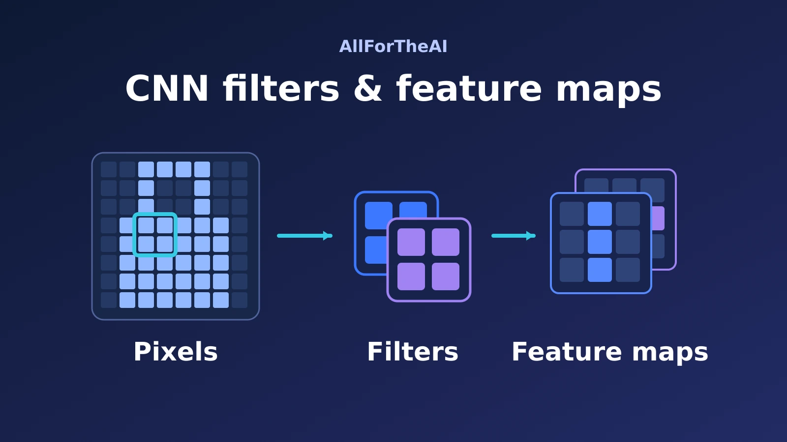
A convolutional neural network (CNN) is a neural network that applies learned filters across local regions of data. For images, those filters create feature maps that highlight useful patterns. Further layers combine the patterns, and a task-specific output layer produces results such as image-class scores.
Imagine a model sorting product photographs into shoes, bags and hats. It receives numbers representing pixels. Convolutional layers transform small neighborhoods of those numbers into useful features, which later layers combine to support a prediction.
CNNs are one family within deep learning. Their filters can also process data beyond photographs, including audio and time series. This guide focuses on images and follows one tiny calculation all the way to a feature map. If weights and layers are unfamiliar, start with Neural Networks Explained.
How filters turn pixels into feature maps
Images and channels
A pixel is one location in an image. A grayscale image can represent each location with one brightness value. A typical color image has three values per location: red, green and blue, called RGB channels.
Think of channels as aligned grids describing the same picture. Width and height describe positions; the channel dimension describes the values available at each position. Later layers also have channels, but their values describe learned features rather than literal colors.
Learned filters and shared weights
A filter, often called a kernel, is a small collection of weights. At each position, it multiplies nearby input values by matching weights, adds the products, and usually adds a learned bias: an adjustable offset.
Repeating that calculation across the image produces a feature map, a grid of responses. Each response is an activation indicating how strongly that filter responds to a particular patch, a small region of the input.
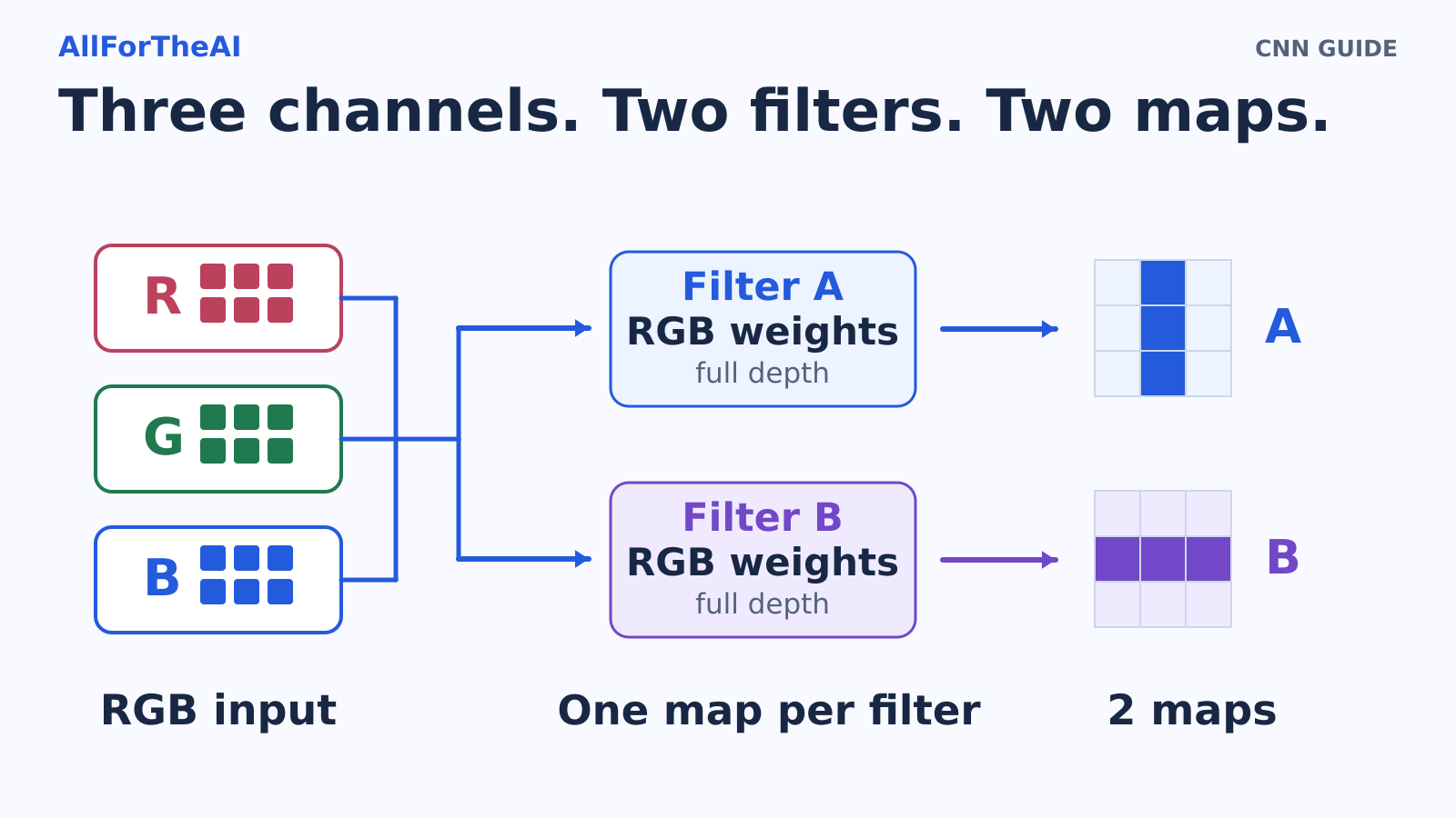
In an ordinary RGB convolution, one filter has weights covering all three input channels. It adds their contributions into one output map. Two filters produce two maps, not six. These maps become two output channels. Grouped and depthwise convolutions use different connection patterns.
The same filter weights are reused at every spatial position. This weight sharing allows the same pattern calculation throughout the picture without learning separate weights for every location. Stanford’s convolutional-network notes explain this local connectivity and sharing. The resulting maps preserve spatial organization, so later layers can combine neighboring responses.
A small CNN filter example you can follow
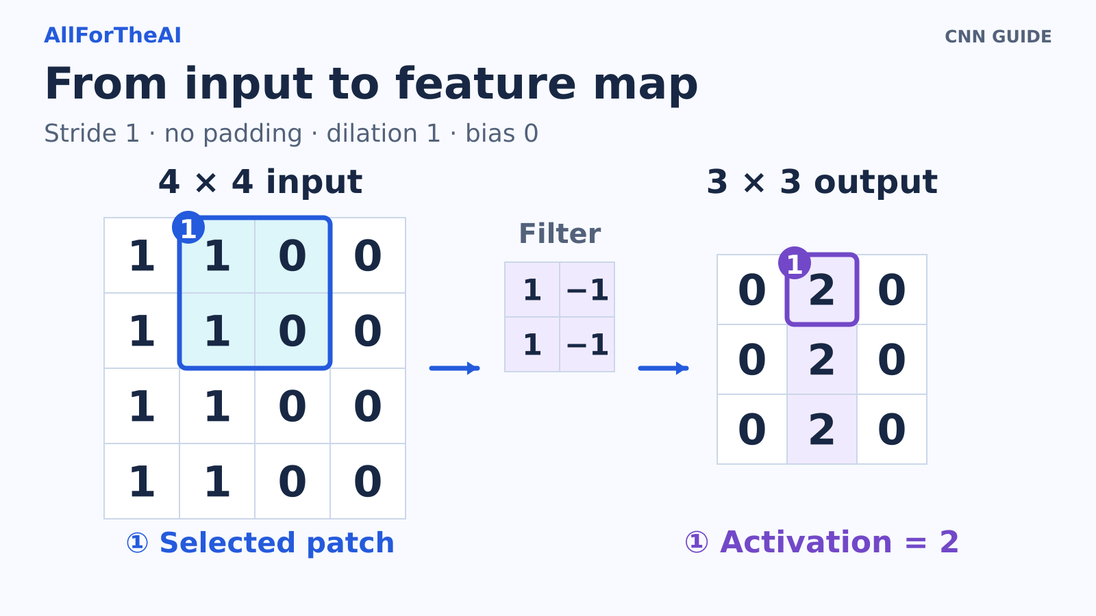
Use this 4 × 4 grayscale image. Each row contains two bright pixels, represented by 1, followed by two dark pixels, represented by 0.
| Row | Col. 1 | Col. 2 | Col. 3 | Col. 4 |
|---|---|---|---|---|
| 1 | 1 | 1 | 0 | 0 |
| 2 | 1 | 1 | 0 | 0 |
| 3 | 1 | 1 | 0 | 0 |
| 4 | 1 | 1 | 0 | 0 |
Choose this 2 × 2 filter for demonstration:
| Row | Col. 1 | Col. 2 |
|---|---|---|
| 1 | 1 | −1 |
| 2 | 1 | −1 |
It is hand-picked, not learned. Use one channel, stride 1, no padding, dilation 1 and zero bias. Here dilation 1 means adjacent filter entries use adjacent pixels. Slide the filter without flipping it. Libraries commonly call this convolution; technically, this operation is cross-correlation, as the PyTorch Conv2d documentation specifies.
Multiply and add one patch
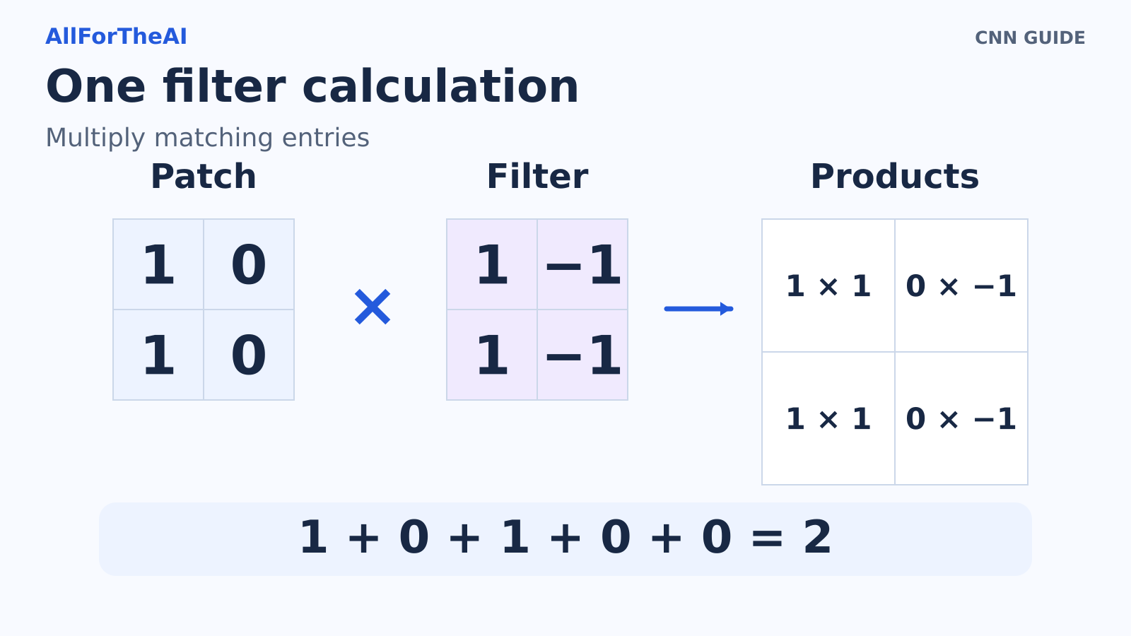
Take rows 1–2 and columns 2–3. Both rows of this patch are [1, 0]. Multiply its four values by the filter’s matching weights, then add:
(1 × 1) + (0 × −1) + (1 × 1) + (0 × −1) + 0 = 2
The final zero is the bias. Put the result in output row 1, column 2. It responds to the left-to-right drop in brightness across this patch. The value 2 is an activation, not a probability or an object label.
Slide the filter to complete the map
The patch one position to the left contains only ones, so its positive and negative products cancel to zero. The patch to the right contains only zeros and also produces zero.
Move down and repeat. Because all input rows are identical, every output row is the same:
| Row | Col. 1 | Col. 2 | Col. 3 |
|---|---|---|---|
| 1 | 0 | 2 | 0 |
| 2 | 0 | 2 | 0 |
| 3 | 0 | 2 | 0 |
There are three valid starting positions horizontally and three vertically. That makes a 3 × 3 map.
Reader check: swap the filter’s two columns. The middle responses become −2, while the other responses remain zero.
What stride and padding change
Stride is the distance between filter positions. Stride 2 moves two pixels per step and produces fewer responses here. Padding adds a border, often zeros, so the filter can extend beyond the original image boundary. Suitable padding can preserve width and height at stride 1.
How CNN layers build a prediction
Nonlinear activation
After convolution, an activation function changes the responses. A common choice is ReLU, short for rectified linear unit: keep positive values and replace negative values with zero.
ReLU leaves our original map unchanged. With the reversed filter, it turns the −2 responses into zeros. This nonlinear step helps stacked layers represent relationships that repeated linear calculations alone cannot. Other activation functions are possible.
Optional downsampling
Downsampling reduces a map’s width and height. One method is max pooling, which keeps the largest value in each local region. Another is convolution with a larger stride.
Smaller maps can reduce later computation, but lose spatial detail. Pooling is optional, and downsampling need not follow every convolution. A task requiring precise locations may need to preserve or recover finer detail.
Combining features and producing class scores
Later convolutions process feature maps rather than raw pixels. Stacking layers lets a response depend on a wider region of the original image. Features can become more useful for the task, without following a guaranteed sequence of edges, eyes and faces.
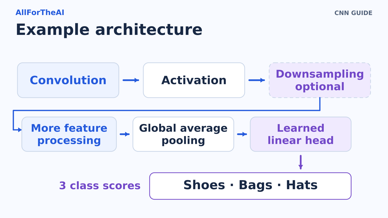
One example classifier follows this path:
Convolution → activation → optional downsampling → more feature processing → global average pooling → learned classification head.
Global average pooling averages each final feature map into one number. A learned linear head combines those numbers into class scores, sometimes called logits. For shoes, bags and hats, it produces three scores.
For a single-label task, where each image receives one class, softmax can turn the scores into probabilities that sum to one. A high probability still does not guarantee a correct prediction. This is one possible architecture, not a required CNN template.
How a CNN learns its filters
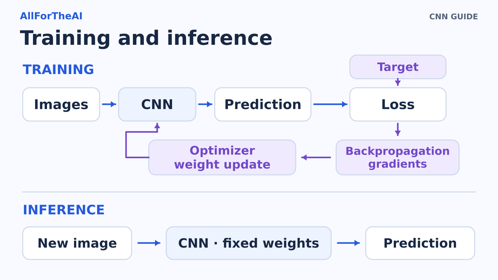
The demonstration filter was chosen to make the arithmetic clear. In a trained classifier, filters and the classification head are normally learned together from examples.
For supervised training, the model predicts classes for a batch of labeled images. A loss function measures how well those predictions match the labels. Backpropagation calculates gradients, numbers describing how small parameter changes would affect the loss. An optimizer uses them to update the trainable weights and biases with the aim of reducing the loss.
Repeating this process can produce useful filters; nobody needs to program a separate rule for every shape. The PyTorch optimization tutorial separates prediction, loss calculation, gradients and parameter updates.
Ordinary inference applies the learned parameters to a new image without updating them. A model can also start from pretrained weights, already learned on another dataset, and be adapted through transfer learning. For the fuller training explanation, continue with How Deep Learning Works.
What CNNs can do and where they can fail
A product-image classifier assigns a category to a photograph. A CNN can also supply features to an object detection system that identifies objects and predicts bounding boxes around them. Those outputs require a suitable task-specific design and training objective.
CNNs operate within the wider field of computer vision. Vision transformers can support many of the same tasks through a different architecture.
Useful filters do not guarantee reliable results. A product classifier might learn that bags usually appear on white backgrounds, then fail when customers photograph them outdoors. This illustrates shortcut learning: relying on an easy association that breaks under different conditions.
Changes in lighting, cameras or products can create distribution shift, meaning new inputs differ from the training data. Poor labels and unrepresentative examples also limit performance. Larger inputs and models demand more memory and computation. Evaluation should therefore use unseen images resembling the intended use, rather than relying only on training performance.
Frequently asked questions
What makes a CNN different from a fully connected network?
A standard convolutional layer connects to local regions and shares filter weights across positions. A fully connected layer connects each output unit to every input value. CNN classifiers can still include fully connected layers in their output head.
Are filters chosen by a programmer or learned during training?
Programmers usually choose settings such as filter size and filter count. Training adjusts the weights inside those filters. Hand-designed filters, like this article’s example, help explain the calculation but do not show the learning process.
What is the difference between a filter and a feature map?
A filter contains weights used for a calculation. A feature map contains the resulting responses across an input. Applying the same filter to two different images usually produces different feature maps, even when its weights stay fixed.
How does a CNN process the three color channels of an image?
In ordinary convolution, each filter covers red, green and blue channels and combines their weighted contributions into one output map. Several filters produce several maps. The output channel count therefore follows the filter count, not the three input colors.
What do stride and padding change?
Stride controls how far the filter moves between calculations. Padding adds values around the input boundary. Together with filter size and dilation, they determine which positions are processed and the resulting feature map’s width and height.
Does every CNN need ReLU and pooling?
No. ReLU is a common activation, but alternatives exist. Pooling is one way to reduce spatial size; strided convolutions can also do this. The exact layers depend on the model and task.
Does a CNN learn again every time it sees a new image?
Usually no. During ordinary inference, the network computes an output using fixed learned parameters. Updating those parameters requires a training or adaptation process; receiving a new image alone does not trigger learning.
Is a CNN the same as image classification or object detection?
A CNN is a model architecture. Image classification and object detection are tasks with different outputs. Either task can use CNN-based models or other architectures, provided the model and training process suit the required output.
Have vision transformers made CNNs obsolete?
No. ConvNeXt research demonstrates competitive convolutional models across vision benchmarks. Choosing between CNNs, transformers and combinations requires testing against the relevant data, accuracy needs, hardware and latency constraints. There is no universal winner.
Key takeaway and where to learn next
A CNN applies shared filters locally, builds learned representations through layers, and produces an output designed for its task. Continue with Image Classification Explained to connect these mechanics to a practical prediction problem, or follow the established Deep Learning → Neural Networks → How Deep Learning Works path for foundations.